Counterfactuals provide a model-agnostic method for black box machine learning algorithms interpretable and human-understandable. Counterfactuals provide explanations as to what the model would have predicted if the inputs were perturbed in a particular way. A counterfactual explanation, therefore, provides a casual description linking model inputs $X$ and predictions $Y$: “If X had not occurred, Y would not have occurred”. For example, “if I had woken up 5 minutes earlier I would have caught the train” is a counterfactual in which wakeup time $X$ is altered to change the outcome $Y=\mathrm{‘Train}$ to $Y=\mathrm{Train}$. Consider the black box model below which takes three input observations $[x_1, x_2, x_3]$ and makes a prediction $Y$:

The causality here is clear, the outcome of the model $Y$ is determined by how the model evaluates the inputs $[x_1, x_2, x_3]$. Counterfactuals make use of this causality: altering the inputs to cause a change in the output. With the most simple methods for finding counterfactuals, we do not need to peak inside the model, instead, we can phrase the search for counterfactuals as an optimisation problem.

Wachter et al. first proposed counterfactual explanations in 2017 as an optimisation problem with two terms:

$$ L(x,x^\prime,y^\prime,\lambda)=\lambda\cdot(f(x^\prime)-y^\prime)^2+D(x,x^\prime) $$

where $x’$ is the counterfactual to the observation $x$, $y'$ is the desired outcome (e.g. caught the train). The first term is a quadratic distance between the model prediction $f(x^\prime)$ and $y'$, which is minimised when $x'$ has been altered sufficiently so that the model predicts $y'$. The second term $D()$ is the more interesting one and reveals more about specifying good counterfactuals:

$$ D(x,x^\prime)=\sum_{j=1}^p\frac{\left|x_j-x^\prime_j\right|}{\mathrm{MAD}_j} $$

The distance metric $D(x,x^\prime)$ measures the distance between each of the $p$ features of $x'$ and $x$ normalised by the median absolute deviation (MAD) of each feature $j$. That we include a distance metric at all indicates, that we want counterfactuals that are relatively close to the original $x$, it’s no use telling me to wake up two hours earlier if I would have got the train being 5 minutes earlier. This feature has the use that it makes counterfactuals reasonable: relying on small changes. The L1 norm has the advantage of promoting sparse solutions in $x'$. Sparsity here is highly desirable because it promotes counterfactuals in which only a small number of variables are changed. This makes the counterfactual easier to interpret and communicate; simply put its makes them descriptively shorter too. Normalising by the MAD places each feature on the same scale, and is more robust to outliers than normalising by the variance $\sigma^2$. The hyperparameter $\lambda$ balances the two terms, with a higher $\lambda$ preferring counterfactuals that better match the desired outcome.

Counterfactuals with sklearn models

To demonstrate counterfactuals we’ll train a simple sklearn classifier on some data. We’ll use the classic breast cancer dataset packaged with sklearn and only use the first two features (mean radius, mean texture) to make the problem easier to visualise. Let’s also train an RBF support vector machine classifier on it:

import numpy as np 
import matplotlib.pyplot as plt
from matplotlib.patches import ConnectionPatch
from sklearn.datasets import load_breast_cancer
from sklearn.svm import SVC
data = load_breast_cancer()
Y = data.target
X = data.data[:, 0:2]
classifier =  SVC(C=.5, probability=True)
classifier.fit(X, Y)

To understand a bit more about the data and how our classifier works let’s plot the dataset and the probability that the growth is cancerous with mean radius and mean texture.

def plot_probability_surface(classifier, levels=20, points=True):
    xx, yy = np.meshgrid(np.linspace(5, 30, 500), np.linspace(5, 45, 500))
    Z = classifier.predict_proba(np.c_[xx.ravel(), yy.ravel()])[:, 1]
    Z = Z.reshape(xx.shape)
    fig, axis = plt.subplots(1, 1, figsize=(10, 10))
    axis.contourf(xx, yy, Z, alpha=0.75, cmap='bone', vmin=0, vmax=1, levels=levels)
    if points:
        axis.scatter(X[:, 0], X[:, 1], c=Y, s=15,
                    cmap='bone', edgecolors='black', linewidth=.5)
    axis.axis('off')
    return axis
ax = plot_probability_surface(classifier)

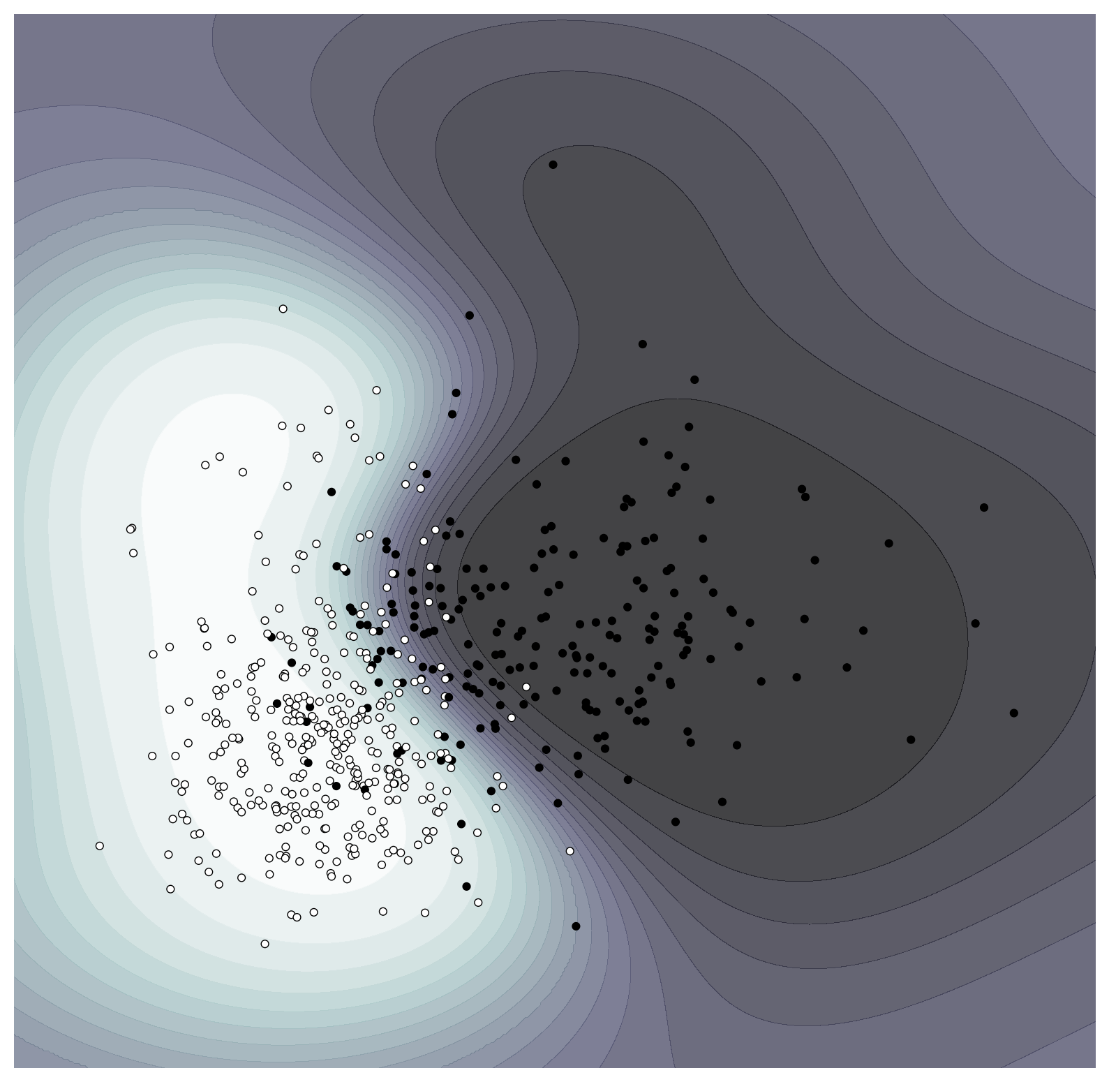
Points plotted in black correspond to those that were identified as malignant while those in white were benign. The classifier has done an acceptable job of learning the overall split in the data, albeit with quite a few outliers. Let’s now define the cost function for evaluating counterfactuals:

import scipy.stats 
def cost_function(x_prime, x, y_prime, lambda_value, model, X):
    mad =  scipy.stats.median_abs_deviation(X, axis=0)
    distance = np.sum(np.abs(x-x_prime)/mad)
    misfit = (model(x_prime, y_prime)-y_prime)**2
    return lambda_value * misfit + distance

We can see that minimising this cost function minimises both the distance of the counterfactual $x'$ to the original observation $x$ through distance, and the misfit to the target prediction $y'$. The function model() is a simple wrapper around the sklearn API to only return the predicted probability:

def evaluate_model(x, y_prime):
    # round the y_prime value to provide the right class [0,1]
    predicted_prob = classifier.predict_proba(x.reshape((1, -1)))[0,int(np.round(y_prime))]
    return predicted_prob

Let’s now detail how to optimise both $\lambda$ and the counterfactual $x'$. For different datasets and models, the optimal $\lambda$ will be different, the optimal $\lambda$ will in fact vary with whatever instance $x$ we attempt to generate a counterfactual for. Because of this the simplest thing to do is to split the optimisation and conduct a line-search over $\lambda$, where we optimise the cost function at different values of $\lambda$ between a range [$\lambda_{min}, \lambda_{max}$].

Given that we might not be able to generate a counterfactual $x'$ for a value of $\lambda$ that minimises $L$ we can evaluate whether the prediction falls within an acceptable tolerance $|f(x')-y'|\leq\epsilon$ to consider it a valid counterfactual explanation.

def get_counterfactuals(x, y_prime_target, model):
    eps = .05 # tolerance
    lambda_min =  1e-10
    lambda_max = 1e4
    lambda_steps = 30
    lambdas = np.logspace(np.log10(lambda_min), 
                            np.log10(lambda_max), 
                            lambda_steps)
    # scan over lambda
    candidates = []
    Y_primes = []
    for lambda_k in lambdas:
        arguments = x, y_prime_target, lambda_k, model, X
        # optimise the cost function -- assuming here it's smooth
        solution = scipy.optimize.minimize(cost_function, 
                                           x, # start from our current observation
                                           args=arguments)
        x_prime_hat = solution.x
        Y_primes.append(model(x_prime_hat, y_prime_target))
        candidates.append(x_prime_hat)
    Y_primes = np.array(Y_primes)
    candidates = np.array(candidates)
    # check if any counterfactual candidates meet the tolerance condition
    eps_condition = np.abs(Y_primes - y_prime_target) <= eps
    return candidates[eps_condition]

Let’s take the following observation as our example which we’ll generate counterfactuals for.

instance = 90
print('mean radius: ',    X[instance, 0], 
      '\nmean texture: ', X[instance, 1], 
      '\ntruth: ',    data.target_names[Y[instance]],
      '\nmodel prediction: ', data.target_names[classifier.predict(X[instance].reshape(1, -1))],
      '\nmodel probability: ', classifier.predict_proba(X[instance].reshape(1, -1)))

mean radius:  14.62 
mean texture:  24.02 
truth:  benign 
model prediction:  ['malignant'] 
model probability:  [[0.87713292 0.12286708]]

So our model has incorrectly classified the benign tumour as malignant. Let’s generate counterfactuals for this observation that would have led to a benign prediction. We’ll focus on a counterfactual that just tips the balance, where the probability $p_{\text{benign}} \approx 0.51$, and with our given tolerance $\epsilon = 0.05$ accept any counterfactuals within $y'\in[0.46, 0.56]$.

P_benign = .51
counterfactuals = get_counterfactuals(X[instance], P_benign, evaluate_model)
counterfactuals

array([[13.34872439, 24.01999999],
       [13.33853873, 24.02077621],
       [13.29875635, 24.01999999],
       [13.30968431, 23.17429894],
       [13.32756653, 23.03365356],
       [13.29820608, 24.02      ]])

Our best counterfactual is that which maximises $\lambda$ which is the last one. We can see that the larger one has a bigger change to the mean radius but does not change the mean texture. As discussed above, if our model had many more features than here, having sparse counterfactuals is preferable for explanatory purposes. We explain the counterfactual as “if the mean radius of the tumour was 9% smaller than the model would have predicted the tumour to have been benign'.

best_counterfactual = counterfactuals[-1]
print("% difference (x', x):", (100*(best_counterfactual-X[instance])/X[instance]).round(2))

% difference (x', x): [-9.04 -0.  ]

ax = plot_probability_surface(classifier, levels=20, points=True)
ax.scatter(X[instance][0], X[instance][1], s=25, fc='None', edgecolors='r', linewidth=2)
ax.plot(best_counterfactual[0], best_counterfactual[1], 'go', markersize=5)
con = ConnectionPatch(X[instance], best_counterfactual, "data", "data",
                      arrowstyle="-|>", shrinkA=5, shrinkB=5,
                      mutation_scale=20, color="red")
ax.add_artist(con)

If we wanted a higher confidence in the prediction, we could see what counterfactual would generate a $p_{\text{benign}}\approx 0.9$.

P_benign = .9
counterfactuals = get_counterfactuals(X[instance], P_benign, evaluate_model)
best_counterfactual = counterfactuals[-1]
print("% difference (x', x):", (100*(best_counterfactual-X[instance])/X[instance]).round(2))
ax = plot_probability_surface(classifier, levels=20, points=True)
ax.scatter(X[instance][0], X[instance][1], s=25, fc='None', edgecolors='r', linewidth=2)
ax.plot(best_counterfactual[0], best_counterfactual[1], 'go', markersize=10)
con = ConnectionPatch(X[instance], best_counterfactual, "data", "data",
                      arrowstyle="-|>", shrinkA=5, shrinkB=5,
                      mutation_scale=20, color="r")
ax.add_artist(con)

% difference (x', x): [-21.15  -0.  ]

Further Reading

• Counterfactual Explanations for Machine Learning: A Review
• Christoph Molnar excellent book Interpretable Machine Learning
• I would recommend the python library Alibi for machine learning model inspection and interpretation, it’s got counterfactual methods built in too.