Visualising 2 billion pixel rasters with datashader and xarray
This post looks at visualising large raster datasets with Datashader and xarray.
Datashader is a python package for visualising large datasets through rasterisation. Linked with other modern python packages such as dask and xarray allow for larger-than-memory dataset processing and distributed computing and visualisation of TB datasets.
The data
The data to visualise is a scientific dataset with satellite observations from the NASA MODIS instruments. A dataset of vegetation leaf area index (LAI) – essentially the average number of leaves on the trees recorded by the instrument is provided in the MCD15 data product.
The raster dataset is provided as smaller datasets split into geographic tiles to make the size more manageable – the data is collected globally at 500 metres! So the observations are split into individual files which correspond to geographic tiles of about 1200km in size. This format is referred to as the MODIS grid and is shown in the image below:
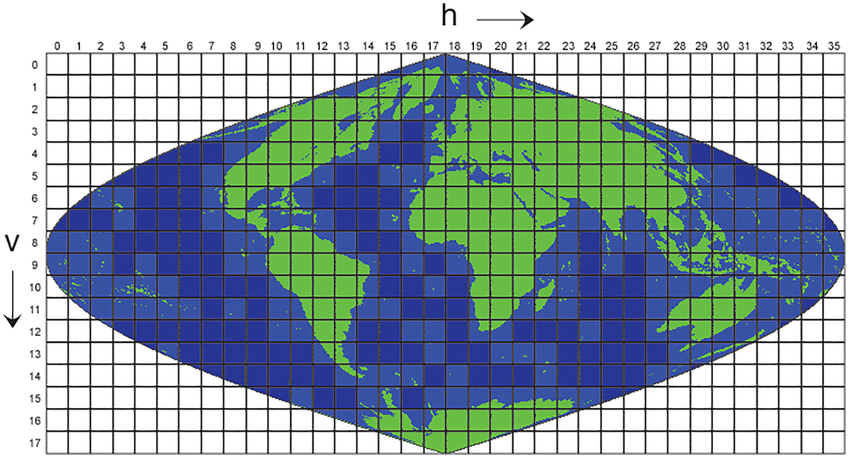
To produce a visualisation covering the entire land surface means dealing with some ~270 individual products which comprise the global product.
$ ls MCD15A2H.A2019001.*
    MCD15A2H.A2019001.h00v08.006.2019014203755.hdf  MCD15A2H.A2019001.h14v10.006.2019014203827.hdf  MCD15A2H.A2019001.h24v02.006.2019014203845.hdf
    MCD15A2H.A2019001.h00v09.006.2019014203829.hdf  MCD15A2H.A2019001.h14v11.006.2019014203821.hdf  MCD15A2H.A2019001.h24v03.006.2019014203846.hdf
    MCD15A2H.A2019001.h00v10.006.2019014203819.hdf  MCD15A2H.A2019001.h14v14.006.2019014203820.hdf  MCD15A2H.A2019001.h24v04.006.2019014203839.hdf
    MCD15A2H.A2019001.h01v07.006.2019014203822.hdf  MCD15A2H.A2019001.h15v02.006.2019014204009.hdf  MCD15A2H.A2019001.h24v05.006.2019014203750.hdf
    MCD15A2H.A2019001.h01v08.006.2019014203812.hdf  MCD15A2H.A2019001.h15v03.006.2019014203825.hdf  MCD15A2H.A2019001.h24v06.006.2019014203834.hdf
    MCD15A2H.A2019001.h01v09.006.2019014203914.hdf  MCD15A2H.A2019001.h15v05.006.2019014203819.hdf  MCD15A2H.A2019001.h24v07.006.2019014203840.hdf
    MCD15A2H.A2019001.h01v10.006.2019014203752.hdf  MCD15A2H.A2019001.h15v07.006.2019014204008.hdf  MCD15A2H.A2019001.h24v12.006.2019014203901.hdf
    ......
    MCD15A2H.A2019001.h14v03.006.2019014203900.hdf  MCD15A2H.A2019001.h23v09.006.2019014203850.hdf  MCD15A2H.A2019001.h35v10.006.2019014203908.hdf

$ ls MCD15A2H.A2019001.* | wc -l
    274
So as expected the data is cut into each tile and stored in a separate file with A2019001 referring to the date of the product (1st January 2019) and the tile such as h15v07. Each is stored as a hdf file which provides several nice features. Given this is geospatial raster data, we’ll use GDAL to interpret and pre-process the data. Let’s use the gdalinfo to look inside one of these:
$ gdalinfo MCD15A2H.A2019001.h13v12.006.2019014203752.hdf

Driver: HDF4/Hierarchical Data Format Release 4
Files: MCD15A2H.A2019001.h13v12.006.2019014203752.hdf
Size is 512, 512
Metadata:
  ALGORITHMPACKAGEACCEPTANCEDATE=10-01-2004
  ALGORITHMPACKAGEMATURITYCODE=Normal
  ALGORITHMPACKAGENAME=MCDPR_15A2

    ⋮
    ⋮
    ⋮

  TileID=51013012
  UM_VERSION=U.MONTANA MODIS PGE34 Vers 5.0.4 Rev 4 Release 10.18.2006 23:59
  VERSIONID=6
  VERTICALTILENUMBER=12
  WESTBOUNDINGCOORDINATE=-65.2703644573188
Subdatasets:
  SUBDATASET_1_NAME=HDF4_EOS:EOS_GRID:"MCD15A2H.A2019001.h13v12.006.2019014203752.hdf":MOD_Grid_MOD15A2H:Fpar_500m
  SUBDATASET_1_DESC=[2400x2400] Fpar_500m MOD_Grid_MOD15A2H (8-bit unsigned integer)
  SUBDATASET_2_NAME=HDF4_EOS:EOS_GRID:"MCD15A2H.A2019001.h13v12.006.2019014203752.hdf":MOD_Grid_MOD15A2H:Lai_500m
  SUBDATASET_2_DESC=[2400x2400] Lai_500m MOD_Grid_MOD15A2H (8-bit unsigned integer)
  SUBDATASET_3_NAME=HDF4_EOS:EOS_GRID:"MCD15A2H.A2019001.h13v12.006.2019014203752.hdf":MOD_Grid_MOD15A2H:FparLai_QC
  SUBDATASET_3_DESC=[2400x2400] FparLai_QC MOD_Grid_MOD15A2H (8-bit unsigned integer)
  SUBDATASET_4_NAME=HDF4_EOS:EOS_GRID:"MCD15A2H.A2019001.h13v12.006.2019014203752.hdf":MOD_Grid_MOD15A2H:FparExtra_QC
  SUBDATASET_4_DESC=[2400x2400] FparExtra_QC MOD_Grid_MOD15A2H (8-bit unsigned integer)
  SUBDATASET_5_NAME=HDF4_EOS:EOS_GRID:"MCD15A2H.A2019001.h13v12.006.2019014203752.hdf":MOD_Grid_MOD15A2H:FparStdDev_500m
  SUBDATASET_5_DESC=[2400x2400] FparStdDev_500m MOD_Grid_MOD15A2H (8-bit unsigned integer)
  SUBDATASET_6_NAME=HDF4_EOS:EOS_GRID:"MCD15A2H.A2019001.h13v12.006.2019014203752.hdf":MOD_Grid_MOD15A2H:LaiStdDev_500m
  SUBDATASET_6_DESC=[2400x2400] LaiStdDev_500m MOD_Grid_MOD15A2H (8-bit unsigned integer)
Corner Coordinates:
Upper Left  (    0.0,    0.0)
Lower Left  (    0.0,  512.0)
Upper Right (  512.0,    0.0)
Lower Right (  512.0,  512.0)
Center      (  256.0,  256.0)
I’ve omitted some of the metadata but the key information is the Subdatasets field which details the individual variables contained within the file. We’re interested in the LAI field which contains the leaf area index data:
$ gdalinfo HDF4_EOS:EOS_GRID:"MCD15A2H.A2019001.h13v12.006.2019014203752.hdf":MOD_Grid_MOD15A2H:Lai_500m

Driver: HDF4Image/HDF4 Dataset
Files: MCD15A2H.A2019001.h13v12.006.2019014203752.hdf
Size is 2400, 2400

    ⋮
    ⋮
    ⋮

Corner Coordinates:
Upper Left  (-5559752.598,-3335851.559) ( 57d44' 6.10"W, 30d 0' 0.00"S)
Lower Left  (-5559752.598,-4447802.079) ( 65d16'13.31"W, 40d 0' 0.00"S)
Upper Right (-4447802.079,-3335851.559) ( 46d11'16.88"W, 30d 0' 0.00"S)
Lower Right (-4447802.079,-4447802.079) ( 52d12'58.65"W, 40d 0' 0.00"S)
Center      (-5003777.339,-3891826.819) ( 54d56' 5.48"W, 35d 0' 0.00"S)
Band 1 Block=2400x416 Type=Byte, ColorInterp=Gray
  Description = MOD15A2H MODIS/Terra Gridded 500M Leaf Area Index LAI (8-day composite)
  NoData Value=255
  Unit Type: m^2/m^2
  Offset: 0,   Scale:0.1
So this provides information about only the LAI data – most importantly that the data is a [2400x2400] raster image and the geographic extent.
Virtual files with GDAL
To visualise the whole dataset will require that we get data from each file and pass it to datashader for imaging. Arranging each file into its geographic area for this would be quite cumbersome. Instead GDAL can do the heavy lifting given the geographic information contained in each hdf file. We also don’t want to just blindly copy the individual files into one big file and keep this on disk - because why duplicate the data? gdalbuildvrt provides a solution for programmatically storing the processing of these individual files into one global raster:
$ gdalbuildvrt --help
Usage: gdalbuildvrt [-tileindex field_name]
                    [-resolution {highest|lowest|average|user}]
                    [-te xmin ymin xmax ymax] [-tr xres yres] [-tap]
                    [-separate] [-b band] [-sd subdataset]
                    [-allow_projection_difference] [-q]
                    [-addalpha] [-hidenodata]
                    [-srcnodata "value [value...]"] [-vrtnodata "value [value...]"]
                    [-a_srs srs_def]
                    [-r {nearest,bilinear,cubic,cubicspline,lanczos,average,mode}]
                    [-oo NAME=VALUE]*
                    [-input_file_list my_list.txt] [-overwrite] output.vrt [gdalfile]*

e.g.
  % gdalbuildvrt doq_index.vrt doq/*.tif
  % gdalbuildvrt -input_file_list my_list.txt doq_index.vrt

NOTES:
  o With -separate, each files goes into a separate band in the VRT band.
    Otherwise, the files are considered as tiles of a larger mosaic.
  o -b option selects a band to add into vrt.  Multiple bands can be listed.
    By default all bands are queried.
  o The default tile index field is 'location' unless otherwise specified by
    -tileindex.
  o In case the resolution of all input files is not the same, the -resolution
    flag enable the user to control the way the output resolution is computed.
    Average is the default.
  o Input files may be any valid GDAL dataset or a GDAL raster tile index.
  o For a GDAL raster tile index, all entries will be added to the VRT.
  o If one GDAL dataset is made of several subdatasets and has 0 raster bands,
    its datasets will be added to the VRT rather than the dataset itself.
    Single subdataset could be selected by its number using the -sd option.
  o By default, only datasets of same projection and band characteristics
    may be added to the VRT.

FAILURE: No target filename specified.
So gdalbuildvrt produces a “virtual file”: a set of instructions to GDAL to arrange and mosaic the 200 odd rasters. Let’s use gdalbuildvrt on the products to create a virtual raster LAI.vrt:
$ gdalbuildvrt -sd 2 LAI.vrt MCD15A2H.A2019001.*
0...10...20...30...40...50...60...70...80...90...100 - done.
The created VRT file LAI.vrt is essentially a text-file containing a set of instructions for GDAL to mosaic and project the individual hdf files.
$ cat LAI.vrt | head
VRTDataset rasterXSize="86400" rasterYSize="31200">
  <SRS dataAxisToSRSAxisMapping="1,2">PROJCS["unnamed",GEOGCS["Unknown datum based upon the custom spheroid",DATUM["Not_specified_based_on_custom_spheroid",SPHEROID["Custom spheroid",6371007.181,0]],PRIMEM["Greenwich",0],UNIT["degree",0.0174532925199433,AUTHORITY["EPSG","9122"]]],PROJECTION["Sinusoidal"],PARAMETER["longitude_of_center",0],PARAMETER["false_easting",0],PARAMETER["false_northing",0],UNIT["Meter",1],AXIS["Easting",EAST],AXIS["Northing",NORTH]]</SRS>
  <GeoTransform> -2.0015109353999998e+07,  4.6331271652777122e+02,  0.0000000000000000e+00,  7.7836536376670003e+06,  0.0000000000000000e+00, -4.6331271652778770e+02</GeoTransform>
  <VRTRasterBand dataType="Byte" band="1">
    <NoDataValue>255</NoDataValue>
    <Scale>0.1</Scale>
    <ColorInterp>Gray</ColorInterp>
    <ComplexSource>
      <SourceFilename relativeToVRT="0">HDF4_EOS:EOS_GRID:"MCD15A2H.A2019001.h00v08.006.2019014203755.hdf":MOD_Grid_MOD15A2H:Lai_500m</SourceFilename>
      <SourceBand>1</SourceBand>

$ cat LAI.vrt | tail

    <ComplexSource>
      <SourceFilename relativeToVRT="0">HDF4_EOS:EOS_GRID:"MCD15A2H.A2019001.h35v10.006.2019014203908.hdf":MOD_Grid_MOD15A2H:Lai_500m</SourceFilename>
      <SourceBand>1</SourceBand>
      <SourceProperties RasterXSize="2400" RasterYSize="2400" DataType="Byte" BlockXSize="2400" BlockYSize="416" />
      <SrcRect xOff="0" yOff="0" xSize="2400" ySize="2400" />
      <DstRect xOff="84000" yOff="19200" xSize="2400" ySize="2400" />
      <NODATA>255</NODATA>
    </ComplexSource>
  </VRTRasterBand>
</VRTDataset>
In this case the file is fairly simple to decipher (well atleast bits). Each file is a ComplexSource and the subdataset for each file isolated as HDF4_EOS:EOS_GRID:"MCD15A2H.A2019001.h35v10.006.2019014203908.hdf":MOD_Grid_MOD15A2H:Lai_500m.
<SrcRect xOff="0" yOff="0" xSize="2400" ySize="2400" /> indicates where to get the input (Src) data in the file and <DstRect xOff="84000" yOff="19200" xSize="2400" ySize="2400" /> explains where to place this data in the virtual file. In this case 19200 pixels down and 84000 across. The VRT file therefore provides a virtual representation of the MODIS tile grid shown in the image above.
And like with the hdf files, gdalinfo provides information on the newly created vrt:
$ gdalinfo LAI.vrt
Driver: VRT/Virtual Raster
Files: LAI.vrt
Size is 86400, 31200
Coordinate System is:
PROJCRS["unnamed",
    BASEGEOGCRS["Unknown datum based upon the custom spheroid",
        DATUM["Not_specified_based_on_custom_spheroid",
            ELLIPSOID["Custom spheroid",6371007.181,0,
                LENGTHUNIT["metre",1,
                    ID["EPSG",9001]]]],
        PRIMEM["Greenwich",0,
            ANGLEUNIT["degree",0.0174532925199433,
                ID["EPSG",9122]]]],
    CONVERSION["unnamed",
        METHOD["Sinusoidal"],
        PARAMETER["Longitude of natural origin",0,
            ANGLEUNIT["degree",0.0174532925199433],
            ID["EPSG",8802]],
        PARAMETER["False easting",0,
            LENGTHUNIT["Meter",1],
            ID["EPSG",8806]],
        PARAMETER["False northing",0,
            LENGTHUNIT["Meter",1],
            ID["EPSG",8807]]],
    CS[Cartesian,2],
        AXIS["easting",east,
            ORDER[1],
            LENGTHUNIT["Meter",1]],
        AXIS["northing",north,
            ORDER[2],
            LENGTHUNIT["Meter",1]]]
Data axis to CRS axis mapping: 1,2
Origin = (-20015109.353999998420477,7783653.637667000293732)
Pixel Size = (463.312716527771215,-463.312716527787700)
Corner Coordinates:
Upper Left  (-20015109.354, 7783653.638) (166d17' 5.25"W, 70d 0' 0.00"N)
Lower Left  (-20015109.354,-6671703.118) (  0d 0' 0.00"E, 60d 0' 0.00"S)
Upper Right (20015109.354, 7783653.638) (166d17' 5.25"E, 70d 0' 0.00"N)
Lower Right (20015109.354,-6671703.118) (  0d 0' 0.00"W, 60d 0' 0.00"S)
Center      (      -0.000,  555975.260) (  0d 0' 0.00"W,  5d 0' 0.00"N)
Band 1 Block=128x128 Type=Byte, ColorInterp=Gray
  NoData Value=255
  Offset: 0,   Scale:0.1
So LAI.vrt has one raster band, a scaling factor to rescale the data to fall between 0.0-2.55 rather than 0-255 which match the expected units of LAI itself. The size of the raster is 86400 pixels “tall” and 31200 pixels wide, which means it contains 2695680000 pixels – i.e some ~2.69 billion!
xarray for out-of-memory rasters
Loading LAI.vrt is remarkably simple thanks to the xarray and rasterio python package which is built on top of GDAL.
import xarray as xr

In [2]: da = xr.open_rasterio("LAI.vrt")

In [3]: da
Out[3]:
<xarray.DataArray (band: 1, y: 31200, x: 86400)>
[2695680000 values with dtype=uint8]
Coordinates:
  * band     (band) int64 1
  * y        (y) float64 7.783e+06 7.783e+06 7.782e+06 ... -6.671e+06 -6.671e+06
  * x        (x) float64 -2.001e+07 -2.001e+07 ... 2.001e+07 2.001e+07
Attributes:
    transform:   (463.3127165277712, 0.0, -20015109.354, 0.0, -463.3127165277...
    crs:         +proj=sinu +lon_0=0 +x_0=0 +y_0=0 +R=6371007.181 +units=m +n...
    res:         (463.3127165277712, 463.3127165277877)
    is_tiled:    1
    nodatavals:  (255.0,)
    scales:      (0.1,)
    offsets:     (0.0,)
Crucially though, xarray has recognised that the LAI.vrt is actually a file composed of many smaller files which chunked together make the fall raster. The is_tiled: 1 attribute means that xarray knows that essentially every 2400x2400 pixels correspond to a new hdf file which needs to be read into memory and processed. This means that xarray can optimise opening only files needed to visualise a certain area, for example only opening files which cover South America. This also means that the whole 2 billion pixels do not need to be simultaneously read into memory. Though in reality, 2.69bn bytes is only ~3Gb.
In [4]: da.nbytes / 1e+9
   ...:
Out[4]: 2.69568
xarray DataArrays behave similarly to numpy arrays, with fancy slice indexing:
In [5]: da[0, 8000:12000, 5000:7000]
Out[5]:
<xarray.DataArray (y: 4000, x: 2000)>
[8000000 values with dtype=uint8]
Coordinates:
    band     int64 1
  * y        (y) float64 4.077e+06 4.076e+06 4.076e+06 ... 2.225e+06 2.224e+06
  * x        (x) float64 -1.77e+07 -1.77e+07 -1.77e+07 ... -1.677e+07 -1.677e+07
Attributes:
    transform:   (463.3127165277712, 0.0, -20015109.354, 0.0, -463.3127165277...
    crs:         +proj=sinu +lon_0=0 +x_0=0 +y_0=0 +R=6371007.181 +units=m +n...
    res:         (463.3127165277712, 463.3127165277877)
    is_tiled:    1
    nodatavals:  (255.0,)
    scales:      (0.1,)
    offsets:     (0.0,)
The key difference here is that the array remains stored on disk in the individual hdf files. We’ve not loaded the data into memory until:
In [7]: da[0, 12000:14000, 5000:7000].values
Out[7]:
array([[255, 255, 255, ..., 255, 255, 255],
       [255, 255, 255, ..., 255, 255, 255],
       [255, 255, 255, ..., 255, 255, 255],
       ...,
       [254, 254, 254, ..., 254, 254, 254],
       [254, 254, 254, ..., 254, 254, 254],
       [254, 254, 254, ..., 254, 254, 254]], dtype=uint8)
Visualisation with datashader
import datashader as ds
from datashader import transfer_functions as tf
from datashader import utils
from colorcet import palette
The principle behind datashader is rasterisation of the data and then imaging. So a dataset of points will be first rasterized to produce you guessed it – an xarray.DataArray. Because da is already a raster datashader we provide it directly with raster():
# colors
cmap = palette['kgy']
bg_col = 'black'
ys, xs = int(da.shape[1]*0.02), int(da.shape[2]*0.02)
agg =  ds.Canvas(plot_width=xs, plot_height=ys).raster(da[0],
                  downsample_method='mean')
img = tf.shade(agg, cmap=cmap)
img = tf.set_background(img, bg_col)
utils.export_image(img=img, filename='lai', fmt=".png",
                    background=None)
Which produces the following:
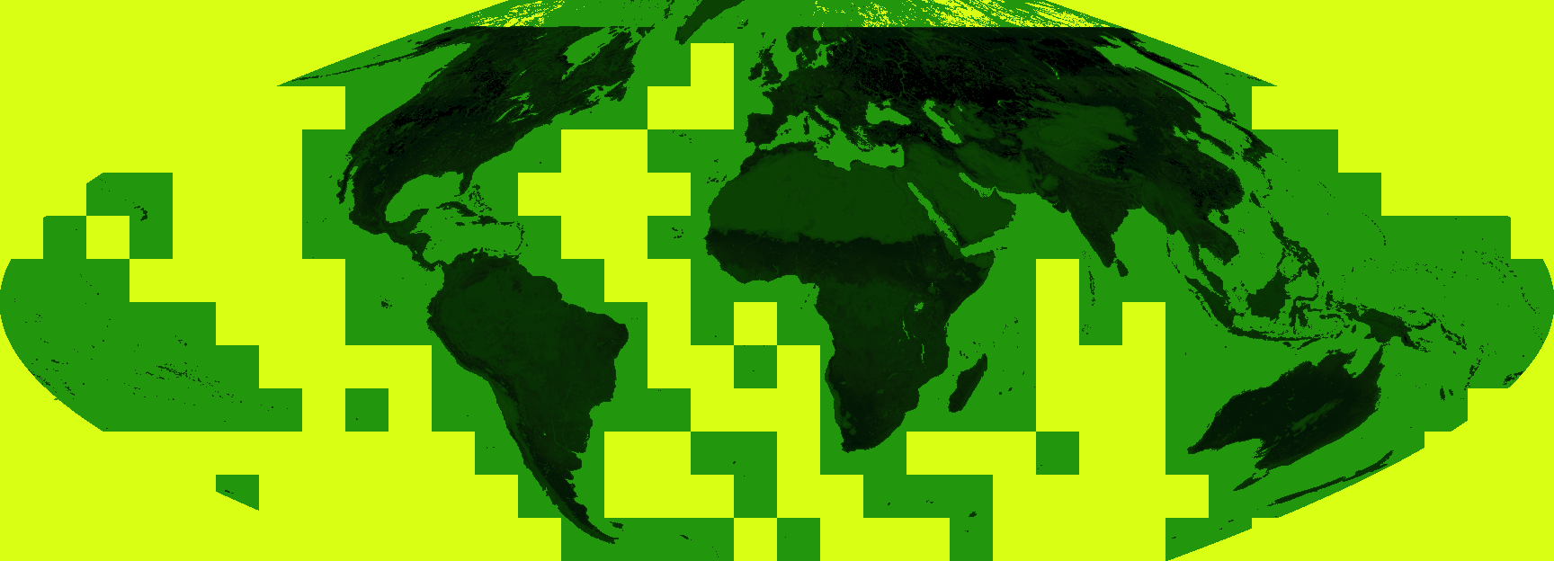
Which is perfectly serviceable – the high LAI areas of the tropics can be made out with the darker greens but the visualisation would be improved by masking out the fill values. Anything greater than 150 (a LAI of 15) is fill:
da = da.where(da < 150.)
agg =  ds.Canvas(plot_width=xs, plot_height=ys).raster(da[0],
                    downsample_method='mean')
img = tf.shade(agg, cmap=cmap)
img = tf.set_background(img, bg_col)
utils.export_image(img=img, filename='lai2', fmt=".png",
                     background=None)
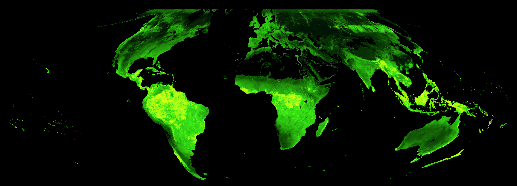
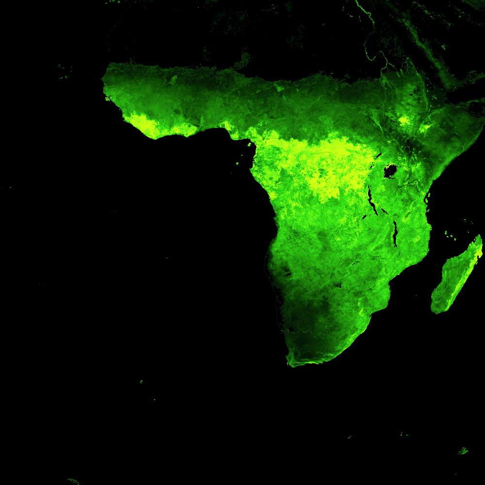
That’s much better! The true areas of highest LAI now pop out in bright green, and the oceans and deserts are now black. It’s also, of course, possible to focus in on one continent to get a better view of detail patterns:
africa = da[0, :, :]
ys, xs = int(africa.shape[1]*0.02), int(africa.shape[2]*0.02)
agg =  ds.Canvas(plot_width=xs, plot_height=ys).raster(africa[0],
                  downsample_method='mean')
img = tf.shade(agg, cmap=cmap)
img = tf.set_background(img, bg_col)
utils.export_image(img=img, filename='lai_africa',
                    fmt=".png", background=None)
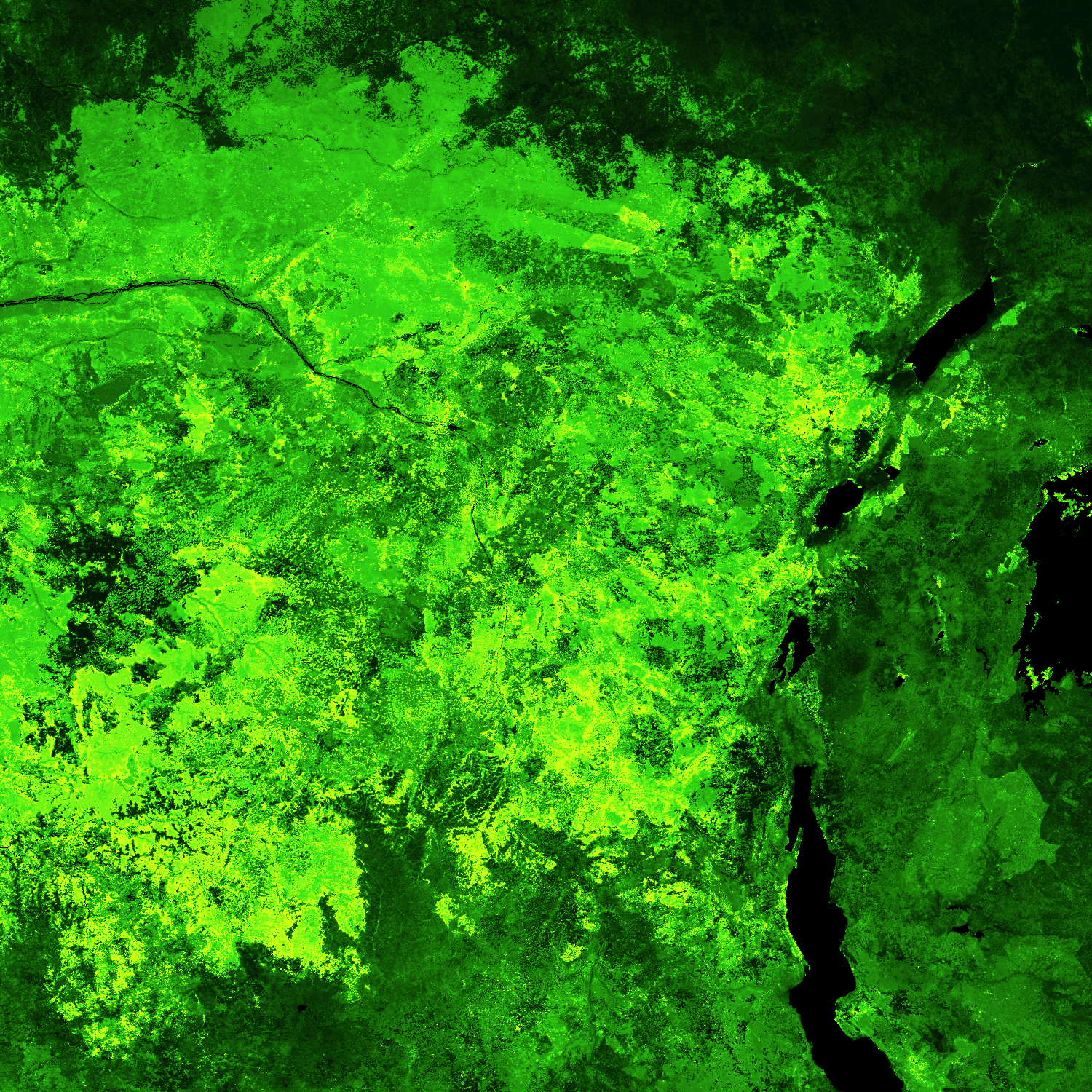
Or zoom into the 500m data even further:
africa_zm = da[0, 15500:18500, 48000:51000]
ys, xs = int(africa_zm.shape[0]*0.5), int(africa_zm.shape[1]*0.5)
agg =  ds.Canvas(plot_width=xs, plot_height=ys).raster(africa_zm,
                downsample_method='mean')
img = tf.shade(agg, cmap=cmap)
img = tf.set_background(img, bg_col)
utils.export_image(img=img, filename='lai_africa_zoom',
              fmt=".png", background=None)