This post looks at estimating empirical cumulative density functions (CDFs) and their confidence intervals from data.

Typically when we have some data an initial exploratory analysis is to consider how our data varies. Lots of the time we might have a good idea of the statistical distribution our data is likely drawn from, measurements collected by a satellite might follow a normal distribution. We could use our data to estimate the moments of the Normal distribution to get our population distribution. Sometimes though we do not have a good idea of whether our distribution follows a parametric distribution and want to turn to non-parametric methods. We do this by estimating the empirical distribution function (the empirical cumulative distribution function CDF) of our data.

To start, we’ll sample some data from our (un)known population:

import scipy.stats
import matplotlib.pyplot as plt
import seaborn as sns
import numpy as np
# create our data
data = scipy.stats.gamma(5,1).rvs(200)

And producing histograms (frequency counts) of the data is super easy of course:

fig, ax = plt.subplots(1,2, figsize=(8, 3))
ax[0].hist(data,lw=1,edgecolor='k')
ax[1].hist(data,lw=1,edgecolor='k', cumulative=True)
[a.set_xlabel("x") for a in ax];
[a.set_ylabel("Frequency") for a in ax];
sns.despine()

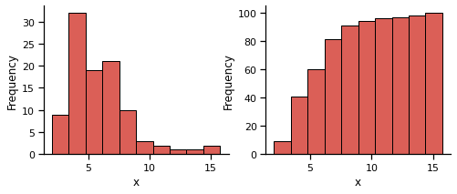
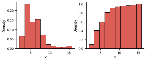
Where the figure on left is an ordinary histogram (i.e. the number of samples in each frequency bin) and the right is the cumulative count of samples for each bin: the cumulative histogram. Of course at the moment these are not strictly empirical distributions until they are normalised to provide discrete probability and cumulative distribution functions:

fig, ax = plt.subplots(1,2, figsize=(8, 3))
ax[0].hist(data, lw=1,edgecolor='k', density=True)
ax[1].hist(data,lw=1,edgecolor='k', cumulative=True, density=True)
[a.set_xlabel("$x$") for a in ax];
[a.set_ylabel("Density") for a in ax];
sns.despine()

The empirical distribution function

Thinking more about how the cumulative density is produced provides a route for not just relying on matplotlib and provides us with a deeper understanding of the quality of our distribution. The empirical distribution function of our data $\hat{F}(x)$ is the cumulative distribution function (CDF) that cumulatively increases by $1/n$ at each data point $X_i$:

$$ \hat{F}(x) = \frac{\sum_{i=1}^{N} \text{I}(X_i \leq x)}{n}$$

where $\text{I}$ provides an indicator function that essentially provides a mathematical function to count the number of samples below $x$:

$$ \text{I}(X_i \leq x) = \begin{cases} 1 & \text{if} & X_i \leq x \\\
0 & \text{if} & X_i > x \end{cases} $$

$X_i$ is less than or equal to the current value of $x$, $\text{I}(X_i)$ equals 1. So at each increment along $x$ we count the number of observations $[X_i \dots X_N]$ that are below or equal to $x$.

Let’s implement this in python and see how it works:

def edf(data):
    x0 = data.min() # get sample space
    x1 = data.max()
    x = np.linspace(x0, x1, 100) 
    N = data.size # number of observations
    y = np.zeros_like(x)
    for i, xx in enumerate(x):
        # sum the vectorised indicator function 
        y[i] = np.sum(data <= xx)/N 
    return x, y

x, y = edf(data)
# plot it
plt.plot(x, y, 'k-')
plt.title("Empirical distribution function - $\hat{F}(x)$")
plt.xlabel("$x$")
plt.ylabel("Density")
plt.plot(data, [0.01]*len(data), '|', color='k')
sns.despine()

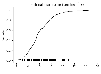
$\hat{F}(x)$ looks at least superficially similar to the cumulative density shown in the plot above, increasing rapidly from 0 and then plateaus as the probabilities reach 1. The plt.plot(data, [0.01]*len(data), '|', color='k') here is a nice trick for indicating sample points as we would with a rugplot.

How good is our distribution? Getting confidence intervals

If we want to get some sort of idea of how constrained our EDF is we want to put some uncertainties on it. Ultimately we want an idea of how far our empirical distribution $\hat{F}(x)$ is from the real unknown CDF $F(x)$.

The Dvoretzky–Kiefer–Wolfowitz (DKW) inequality provides a method to bound the probability of the agreement between $\hat{F}(x)$ and $F(x)$. From the DKW inequality, a non-parametric upper and lower confidence interval that bounds $F(x)$ within ($1-\alpha$) is:

$$ \text{Lower}[\hat{F}(x)] = \text{max} [ \hat{F}(x) - \epsilon, \; 0 ] $$

$$ \text{Upper}[\hat{F}(x)] = \text{min} [ \hat{F}(x) + \epsilon, \; 1 ] $$

where $\epsilon$ is:

$$ \epsilon = \sqrt{ \frac{1}{2n} \text{log}\left(\frac{2}{\alpha}\right)}$$

The direct interpretation of $\epsilon$ is that anywhere along the EDF, the probability that $\hat{F}(x)$ is more than $\epsilon$ away from the true CDF $F(x)$ is:

$$ P(| \hat{F}(x)-{F}(x)| > \epsilon) \leq 2e^{-2n\epsilon^2} $$

Being a concentration inequality, the DKW provides an upper bound on the confidence interval (a looser confidence interval). Adding this to the edf function:

def edf(data, alpha=.05, x0=None, x1=None ):
    x0 = data.min() if x0 is None else x0
    x1 = data.max() if x1 is None else x1
    x = np.linspace(x0, x1, 100)
    N = data.size
    y = np.zeros_like(x)
    l = np.zeros_like(x)
    u = np.zeros_like(x)
    e = np.sqrt(1.0/(2*N) * np.log(2./alpha))
    for i, xx in enumerate(x):
        y[i] = np.sum(data <= xx)/N
        l[i] = np.maximum( y[i] - e, 0 )
        u[i] = np.minimum( y[i] + e, 1 )
    return x, y, l, u

To calculate a 95% confidence interval ($1-0.05$):

x, y, l, u = edf(data, alpha=0.05)
plt.fill_between(x, l, u)
plt.plot(x, y, 'k-')
plt.title("Empirical distribution function - $\hat{F}(x)$")
plt.xlabel("$x$")
plt.ylabel("Density")
plt.plot(data, [0.01]*len(data), '|', color='k')
sns.despine()

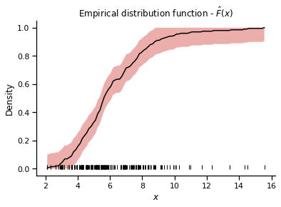
Which shows that our estimated EDF is not too shabby. The confidence intervals really shine however when we consider the impact of the number of samples we have on the EDF:

fig, ax = plt.subplots(2,2, figsize=(8,5),
                             sharex=True, sharey=True, 
                             tight_layout=True)
ax = ax.flatten()
sns.despine()
# make a sample space
xcdf = np.linspace(0, 14)
# try some different N values
Nsamps = np.logspace(1,2, 4).astype(int)
for k, Ns in enumerate(Nsamps):
    data = scipy.stats.gamma(5,1).rvs(Ns)
    # calculate edf
    x, y, l, u = edf(data, x0=0, x1=14)
    ax[k].fill_between(x, l, u)
    ax[k].plot(x, y, 'k-')
    ax[k].set_title(f"Samples: {Ns}")
    ax[k].set_xlabel("$x$")
    ax[k].set_ylabel("Density")
    ax[k].plot(xcdf, scipy.stats.gamma(5,1).cdf(xcdf), 
                'k--', linewidth=1   )
    ax[k].plot(data, [0.01]*len(data), '|', color='k')

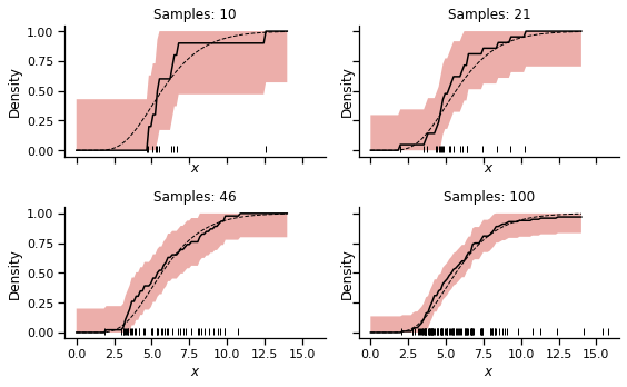
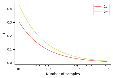
So the width of 95% confidence interval shrinks proportionally to $N$, providing us with a clear measure of the trust we can put in our cumulative distribution. We can get an idea of the width of the confidence interval from considering $\epsilon$ as a function of the number of observations $N$:

N = np.logspace(1, 4)
plt.plot(N, np.sqrt( 1.0/(2*N) *np.log(2./.32)), label='$1\sigma$')
plt.plot(N, np.sqrt( 1.0/(2*N) *np.log(2./.05)), label='$2\sigma$')
plt.semilogx()
plt.ylabel("$\epsilon$")
plt.xlabel("Number of samples")
plt.legend(loc='best')
sns.despine()