Fast and easy gridding of point data with geopandas
This post looks at using the geopandas library to do fast efficient gridding of point data onto a regular grid. Geopandas is a python package that provides a geospatial extension to pandas – so that dataframes can store geographic data such as points and polygons.
Data
A simple csv of point data provides a useful starting point for this. dob.csv contains locations of wildfires detected by the NASA MODIS instruments for a year over North and South America.
import pandas as pd
import numpy as np
import matplotlib.pyplot as plt
df = pd.read_csv("dob.csv", index_col=0)
df = df.sort_values('y')
df = df.drop(columns="geometry")
df.head()
| x | y | dob | |
|---|---|---|---|
| 111 | -5.4247e+06 | -4.38456e+06 | 206 |
| 110 | -5.42516e+06 | -4.38456e+06 | 206 |
| 109 | -5.42238e+06 | -4.38317e+06 | 206 |
| 108 | -5.42284e+06 | -4.38317e+06 | 206 |
| 107 | -5.42794e+06 | -4.38317e+06 | 199 |
So as expected the data is essentially a collection of around 230-thousand x and y points in a projected sinusoidal projection (the MODIS projection) and the day of the year (dob) that the fire occurred.
geopandas
Given our spatial data is point data with x and y coordinates it’s simple to convert the df into a geopandas GeoDataFrame:
import geopandas
gdf = geopandas.GeoDataFrame(df,
            geometry=geopandas.points_from_xy(df.x, df.y),
            crs="+proj=sinu +lon_0=0 +x_0=0 +y_0=0 +a=6371007.181 +b=6371007.181 +units=m +no_defs")
gdf.head()
| x | y | dob | geometry | |
|---|---|---|---|---|
| 111 | -5.4247e+06 | -4.38456e+06 | 206 | POINT (-5424696.941458113 -4384559.892867883) |
| 110 | -5.42516e+06 | -4.38456e+06 | 206 | POINT (-5425160.25417464 -4384559.892867883) |
| 109 | -5.42238e+06 | -4.38317e+06 | 206 | POINT (-5422380.377875471 -4383169.954718296) |
| 108 | -5.42284e+06 | -4.38317e+06 | 206 | POINT (-5422843.690592 -4383169.954718296) |
| 107 | -5.42794e+06 | -4.38317e+06 | 199 | POINT (-5427940.130473807 -4383169.954718296) |
So geopandas has taken the x and y fields and made simple point geometries. We don’t need the x and y fields anymore so let’s drop those and then use geopandas to plot the points:
gdf = gdf.drop(columns=['x', 'y'])
gdf.tail()
| dob | geometry | |
|---|---|---|
| 6 | 197 | POINT (-5506239.979567026 6673324.712505849) |
| 5 | 197 | POINT (-5506703.292283554 6673324.712505849) |
| 4 | 205 | POINT (-5507166.605000081 6673324.712505849) |
| 1 | 191 | POINT (-5510409.794015776 6673324.712505849) |
| 0 | 205 | POINT (-5504850.041417442 6674714.650655435) |
Like pandas, geopandas has built in plotting routines:
gdf.plot(markersize=.1, figsize=(8, 8))
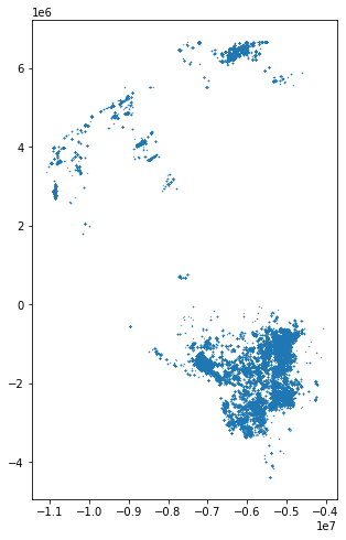
So that doesn’t make a lot of sense yet although geopandas has correctly plotted a marker for each point using the geometry column of the dataframe. Let’s make a more useful plot of the data:
ax = gdf.plot(markersize=.1, figsize=(12, 8), column='dob', cmap='jet')
plt.autoscale(False)
world = geopandas.read_file(geopandas.datasets.get_path('naturalearth_lowres'))
world.to_crs(gdf.crs).plot(ax=ax, color='none', edgecolor='black')
ax.axis('off')
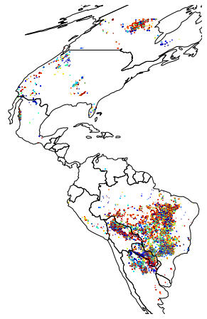
That looks better! A nice feature of geopandas is that it has built on-the-fly reprojection – we’ve taken the world geodataframe and reprojected it from WGS84 to the MODIS sinusoidal projection that the fire data is in with the coordinate reference systems. world.to_crs(gdf.crs)
Gridding with geopandas
Turning to the gridding, geopandas has operations for merging geometries and aggregating statistics to overlapping geometries in ways that will be familiar to pandas users.
First, let’s make the grid that the data is being binned into. To make a regular rectangular mesh for the binned data we can loop over the extent of the data and use shapely to produce each individual grid cell as a geometric polygon:
# total area for the grid
xmin, ymin, xmax, ymax= gdf.total_bounds
# how many cells across and down
n_cells=30
cell_size = (xmax-xmin)/n_cells
# projection of the grid
crs = "+proj=sinu +lon_0=0 +x_0=0 +y_0=0 +a=6371007.181 +b=6371007.181 +units=m +no_defs"
# create the cells in a loop
grid_cells = []
for x0 in np.arange(xmin, xmax+cell_size, cell_size ):
    for y0 in np.arange(ymin, ymax+cell_size, cell_size):
        # bounds
        x1 = x0-cell_size
        y1 = y0+cell_size
        grid_cells.append( shapely.geometry.box(x0, y0, x1, y1)  )
cell = geopandas.GeoDataFrame(grid_cells, columns=['geometry'],
                                 crs=crs)
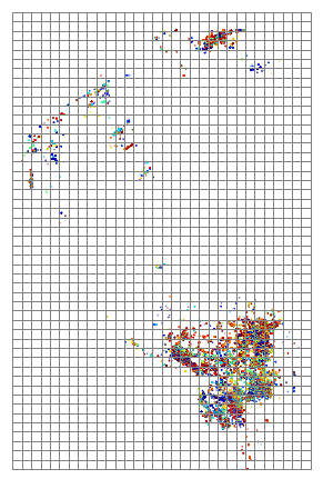
Plotting the grid over the data shows how the fires are generally clustered into a few regions and we’ll end up with many “empty” grid cells:
ax = gdf.plot(markersize=.1, figsize=(12, 8), column='dob', cmap='jet')
plt.autoscale(False)
cell.plot(ax=ax, facecolor="none", edgecolor='grey')
ax.axis("off")
geopandas sjoin and dissolve
Geopandas can then combine geodataframes based on the geometries of each row, in a manner similar to how vanilla pandas merges based on column values.
sjoin is used to merge the two dataframes:
merged = geopandas.sjoin(gdf, cell, how='left', op='within')
so gdf and cell will be merged according to the geometries in cell – eg each grid using the operator rule within – or each row of gdf will be associated with the grid cell that its location falls within.
Now we want to count the number of fires in each grid cell. This can be achieved by aggregating merged so that the number of rows for each grid cell is counted. In geopandas this aggregation process is referred to as dissolving – i.e. making the data more sparse:
# make a simple count variable that we can sum
merged['n_fires']=1
# Compute stats per grid cell -- aggregate fires to grid cells with dissolve
dissolve = merged.dissolve(by="index_right", aggfunc="count")
# put this into cell
cell.loc[dissolve.index, 'n_fires'] = dissolve.n_fires.values
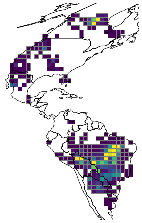
Then finally let’s plot the grid and the number of fires in each grid cell with geopandas:
ax = cell.plot(column='n_fires', figsize=(12, 8), cmap='viridis', vmax=5000, edgecolor="grey")
plt.autoscale(False)
world = geopandas.read_file(geopandas.datasets.get_path('naturalearth_lowres'))
world.to_crs(cell.crs).plot(ax=ax, color='none', edgecolor='black')
ax.axis('off')
r-trees and fast spatial joins
The reason that spatial joins in geopandas are fast is that geopandas leverages a useful data partitioning algorithm – the R-tree. R-trees are data structures which index spatial data in a way that makes identifying data from a spatial region faster than a brute force search approach. An R-tree collects points/geometries nearby each other into a tree-like structure of bounding boxes that define a spatial area that is then a quick method for spatial indexing.
In geopanads, the r-tree is built when the attribute gdf.sindex is accessed:
r_tree = gdf.sindex
print(r_tree)
rtree.index.Index(bounds=[-11105837.471524423, -4384559.892867883, -4067190.682031316, 6674714.650655435], size=226719)
The r-tree has a leaves method which shows the spatial partitioning structure of each leaf of the r-tree:
for leaf in r_tree.leaves()[:2]:
    idxs, indices, bbox = leaf
    print(f'-> points in box {idxs}: ',  indices, '\n bounding box: ', bbox, '\n')
print(f"number of leaves: {len(r_tree.leaves())}")
-> points in box 6:  [182654, 182656, 182665, 182663, 182659, 182664, 182655, 182657, 182660, 182652, 182653, 182675, 182677, 182671, 182670, 182674, 182680, 182678, 182673, 182672, 182669, 182668, 182679, 182676, 182686, 182681, 182684, 182687, 182690, 182688, 182685, 182682, 182689, 182683, 182692, 182696, 182693, 182699, 182695, 182697, 182694, 182691, 182698, 182703, 182702, 182706, 182704, 182707, 182701, 182705, 182700, 182710, 182711, 182709, 182708, 182712, 182713, 182714, 182715, 182716, 182718, 182717, 182719, 182721, 182720, 182722, 182728, 182725, 182724, 182729]
 bounding box:  [-10882520.74215797, 2750455.9416639777, -10852868.728300184, 2759722.1959945355]

-> points in box 7:  [182730, 182723, 182727, 182726, 182741, 182733, 182731, 182740, 182739, 182742, 182734, 182732, 182735, 182738, 182736, 182737, 182743, 182756, 182744, 182754, 182746, 182749, 182750, 182747, 182748, 182753, 182752, 182751, 182755, 182745, 182757, 182758, 182760, 182759, 182762, 182761, 182763, 182764, 182767, 182769, 182766, 182768, 182770, 182765, 182776, 182777, 182774, 182772, 182771, 182775, 182773, 182779, 182781, 182780, 182778, 182782, 182784, 182788, 182786, 182785, 182789, 182787, 182783, 182795, 182797, 182791, 182790, 182794, 182793, 182792]
 bounding box:  [-10869084.67337866, 2759722.1959945355, -10855648.604599353, 2763892.010443287]

number of leaves: 3239
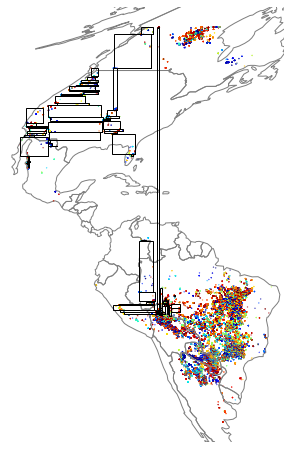
Plotting the first 200 bounding boxes shows how the data is partitioned geographically:
import shapely.geometry
from descartes import PolygonPatch
ax = gdf.plot(markersize=.1, figsize=(12, 8), column='dob', cmap='jet')
plt.autoscale(False)
for leaf in r_tree.leaves()[:200]:
    idxs, indices, bbox = leaf
    r_box = shapely.geometry.box(*bbox)
    box_patch = PolygonPatch(r_box, fc='None', ec='k')
    ax.add_patch(box_patch)
world.to_crs(gdf.crs).plot(ax=ax, color='none', edgecolor='grey')
ax.axis('off')