06 Mar 2021

Horseshoe priors in numpyro

This post looks at how to implement a horseshoe prior in numpyro to do sparse Bayesian inference. We’ll see that the horseshoe prior provides a nicer shrinkage prior than lasso or ridge priors because it’s more concentrated and more flexible.

Let’s start from the classical linear model where we predict a vector of some data $Y$ based on a design matrix $X$ and a vector of model coefficients $\beta$:

$$ Y = X \beta + \epsilon $$

We don’t expect our model to be an exact representation of the data generation process so the model will have some error $\epsilon$.

From regularisation to Bayesian priors

In some cases, we’re drowning in predictors: either we’ve got far too many predictors we think might be involved, or at worse just happened to be in our CSV and we don’t know what do to with them. In extreme cases, the number of rows in $X$ exceeds the number of data points we have in $Y$.

One common frequentist approach to this problem has been through regularisation, in which the cost function $J(\beta)$ is augmented with a regularisation term that penalises larger values of $\beta$ at the expense of a worse fit to the data in what is referred to as ridge regression:

$$ J(\beta) = || X \beta - Y ||^2 + \lambda ||\beta||^2 $$

The term $\lambda ||\beta||^2$ penalises larger $\beta$ in a squared fashion due to the L2 norm, the strength of which is determined by the regularisation hyperparameter $\lambda$. $\lambda ||\beta||^2$ encourages the solution towards smaller values of all $\beta$, alternatively if we expect that some coefficients should be zero we can use an L1 norm in a lasso regression model:

$$ J(\beta) = || X \beta - Y ||^2 + \lambda |\beta| $$

which encourages sparser solutions than the L2 norm and is re.

When we recast these models in a Bayesian sense we can get new insights into how some of the regularisation methods work. Let’s take our unconstrained model, we’ll assume that the errors $\epsilon$ are zero-mean iid normally distributed $\mathcal{N}(0, \sigma^2)$. We can write our predictive model explicitly with this error model:

$$ Y \sim \mathcal{N}(X\beta, \sigma^2) $$

Now our data $Y$ is modelled as a random variable (RV) with a normal distribution for each point $Y_i$ described by a mean $(X \beta)_i$ and variance $\sigma^2$. With Bayesian inference, we extend this principle to encode all of our model parameters to be random variables also. So for our model above this means defining $\beta$ and $\sigma$ as RVs and in some cases $X$ when we have uncertainties in our predictors. For now, let’s not go “turtles all the way down” and only define a prior distribution for $\beta$ and assume $x$ and $\sigma$ known.

In our two regularisation examples, the prior distributions for $\beta$ are explicitly defined by the functionals. We could recast the L1 regularisation into a Bayesian model using a Laplacian prior for $\beta$ and the L2 a normal prior for $\beta$.

The horseshoe

Taking a Bayesian approach gives us more flexibility about how we define our priors, by making it possible to get inferences of mixture model priors that have the right properties for sparsity inducing priors. The Horseshoe prior is one such prior:

$$ \beta_i | \lambda_i, \tau \sim \mathcal{N}(0, \lambda_i^2, \tau^2) $$ $$ \lambda_i \sim C^+(0,1) $$ $$ \tau \sim C^+(0, 1)$$

There’s a lot to unpack here. Each coefficient $\beta_i$ is modelled as a normal distribution with a variance of $\lambda_i^2, \tau^2$. These two terms, define our mixture model, $\lambda_i$ provides a local shrinkage parameter - local to the individual coefficient $\beta_i$. While $\tau$ provides a global shrinkage parameter which is shared across all coefficients. Both shrinkage parameters are defined with a half-Cauchy distribution $C^+(0,1)$ which provide weakly informative priors.

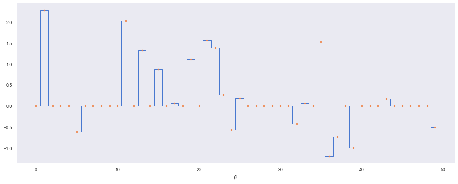
Now let’s use numpyro to detail the benefits of the horseshoe. First, let’s make some data $Y$ we wish to model that has a sparse set of predictors using make_sparse_coded_signal.

import matplotlib.pyplot as plt
import matplotlib
matplotlib.rcParams['figure.figsize'] = (16, 6)
import seaborn as sns 
import numpy as np 
sns.set_style("dark"); sns.set_palette("muted"); sns.set_context("paper")

from sklearn.datasets import make_sparse_coded_signal

y, X, beta = make_sparse_coded_signal(n_samples=1,
                                   n_components=50,
                                   n_features=100,
                                   n_nonzero_coefs=20,
                                   random_state=0)


# add some noise to y
y = y + 0.1 * np.random.randn(len(y))

plt.step(range(len(beta)), beta,  where='mid', lw=1)
plt.plot(range(len(beta)), beta, '.')
plt.xlabel(r'$\beta$')

png

Let’s define our model in numpyro, using plate to split up the indpendent RVs for $\lambda$:

import numpyro
import numpyro.distributions as dist
import jax.numpy as jnp

def horeshoe_linear_model(y=None, X=None, y_sigma=.1):
    n_predictors = X.shape[1]
    Tau = numpyro.sample('tau', dist.HalfCauchy(scale=1))
    with numpyro.plate('local_shrinkage', n_predictors):
        Lambda = numpyro.sample('lambda', dist.HalfCauchy(scale=1))
        horseshoe_sigma = Tau**2*Lambda**2
        Beta = numpyro.sample('beta', dist.Normal(loc=0, scale=horseshoe_sigma))
    mu = jnp.dot(X, Beta)
    numpyro.sample('obs', dist.Normal(loc=mu, scale=y_sigma), obs=y)

And sample from our model using numpyro's built in NUTS sampler:

from numpyro.infer import MCMC, NUTS
from jax import random

nuts_kernel = NUTS(horeshoe_linear_model)
mcmc = MCMC(nuts_kernel, num_warmup=500, num_samples=1000)
rng_key = random.PRNGKey(0)
mcmc.run(rng_key, y=y, X=X)

sample: 100%|██████████| 1500/1500 [00:09<00:00, 152.43it/s, 374 steps of size 2.70e-03. acc. prob=0.86]

We’ll add the expected value of $\beta$ estimated for our model to our spikey plot above:

posterior_samples = mcmc.get_samples()
beta_mu = jnp.mean(posterior_samples['beta'], axis=0)
plt.step(range(len(beta)), beta,  where='mid', lw=1)
plt.plot(range(len(beta)), beta, '.')
plt.plot(range(len(beta)), beta_mu, 'g*')
plt.xlabel(r'$\beta$')

png

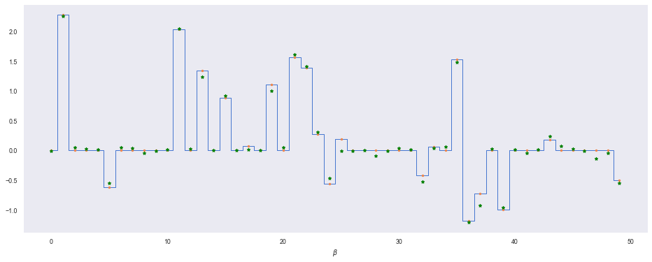
So our model (green dots) does a good job of retrieving a sparse solution that matches well with the true $\beta$. Let’s contrast it with a classic least-squares solution where we have no prior on $\beta$. We can also implement this model in a Bayesian way by using a flat prior over $\beta$ so that we encode no knowledge (or concentration) into the distribution.

def linear_model(y=None, X=None, y_sigma=.1):
    n_predictors = X.shape[1]
    Lambda = numpyro.sample('Lambda', dist.HalfCauchy(scale=1))
    with numpyro.plate('beta_plate', n_predictors):
        Beta = numpyro.sample('beta', dist.Uniform(low=-1000, high=1000))
    mu = jnp.dot(X, Beta)
    numpyro.sample('obs', dist.Normal(loc=mu, scale=y_sigma), obs=y)

lsq_mcmc = MCMC(
            NUTS(linear_model), 
            num_warmup=500, num_samples=1000)
lsq_mcmc.run(random.PRNGKey(0), y=y, X=X)
lsq_samples =  lsq_mcmc.get_samples()


posterior_samples = lsq_mcmc.get_samples()
beta_mu = jnp.mean(posterior_samples['beta'], axis=0)

plt.step(range(len(beta)), beta,  where='mid', lw=1)
plt.plot(range(len(beta)), beta, '.')
plt.plot(range(len(beta)), beta_mu, 'g*')
plt.xlabel(r'$\beta$')

sample: 100%|██████████| 1500/1500 [00:07<00:00, 204.90it/s, 47 steps of size 1.84e-02. acc. prob=0.87]

png

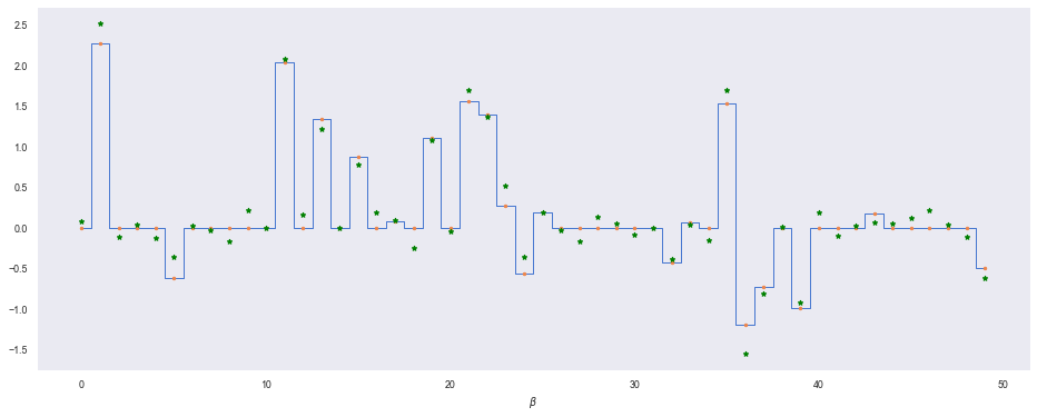
Without any shrinkage, $\beta$ is fitted to residual noise in the dataset (we can see this if we compare $\beta_8$ across both models for example).

James Brennan

Horseshoe priors in numpyro

From regularisation to Bayesian priors

The horseshoe

Further reading