For any model more complex than some well studied examples, an exact description of the posterior is computationally intractable. Beyond an exhaustive evaluation, approximate inference makes it possible to retrieve reasonable descriptions of a posterior or cost surface based on approximation methods. While for many models, Markov chain Monte Carlo is the approximate inference method of choice, the Laplace approximation still provides the simplest deterministic method available.

Simply put the Laplace approximation entails finding a Gaussian approximation to a continuous probability density. Let’s consider a univariate continuous variable $x$ whose distribution $p(x)$ is defined as:

$$ p(z) = \frac{1}{Z}f(z) $$

where $Z$ is the normalisation coefficient

$$Z=\int f(z) \; \mathrm{d} z$$

which ensures the integral of distribution is 1. As with other approximate inference methods, the goal of the Laplace approximation is to find a Gaussian approximation $q(z)$ to the distribution $p(z)$. The mean of this approximation is specified to be the mode of the true distribution $p(z)$, the point $z_0$.

We make a Taylor expansion of $\ln f(z)$ centred on $z_0$ to provide an approximation for $\ln f(z)$:

$$ \ln f(z) \approx \ln f(z_0) - \frac{1}{2}A (z-z_0)^2 $$

where

$$ A = -\frac{\mathrm{d}^2}{\mathrm{d} z^2} \ln f(z) \bigg\rvert_{z=z_0}$$

Taking the exponential of $\ln f(z)$ provides an approximation to our function or likelihood $f(z)$:

$$ f(z) \approx f(z_0) \exp \left[ -\frac{A}{2}(z-z_0)^2 \right] $$

We reach our proper approximate distribution $q(z)$ by making use of the standard normalisation of a Gaussian so that $q(z)$ is:

$$ q(z) = \left(\frac{A}{2\pi}\right)^{1/2} \exp \left[ -\frac{A}{2}(z-z_0)^2 \right] $$

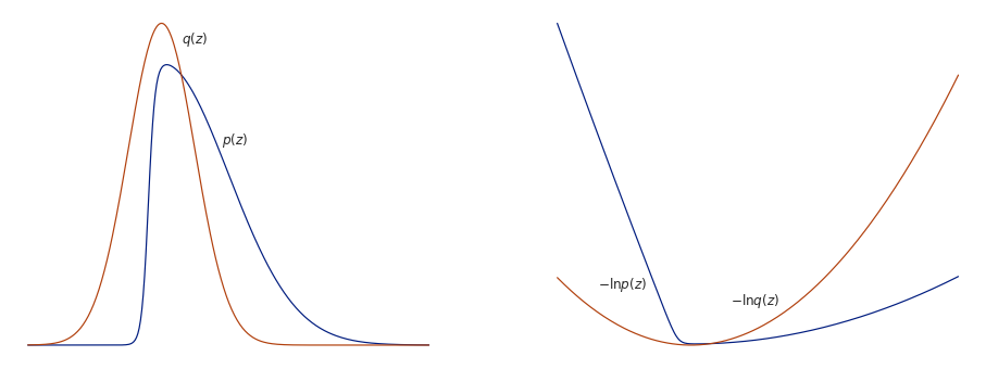
Below illustrates the principle. The asymmetric distribution $q(z)$ can be approximated with a Gaussian distribution $p(z)$. The left figure shows the two distributions with $p(z)$ centred on the mode. The right figure shows the negative logarithms of each distribution, which highlights the inability of the approximation to represent the asymmetry of $q(z)$.

Laplace approximation for multivariate inference

We can of course extend the Laplace approximation for a multivariate distribution. For the $M$-dimensional multivariate distribution $p(\mathbf{z})$, $\mathbf{z}\in R^M$ we can carry out a multivariate procedure. Taking the Taylor expansion at the mode $\mathbf{z}_0$ again:

$$ \ln f(\mathbf{z}) \approx \ln f(\mathbf{z}_0) -\frac{1}{2} (\mathbf{z} - \mathbf{z}_0)^T \mathbf{H} (\mathbf{z} - \mathbf{z}_0) $$

where $\mathbf{H}$ is the Hessian matrix, the matrix of second-order partial derivatives which describes the local curvature of $\ln f(\mathbf{z})$ at $\mathbf{z}_0$. As before exponentiating and including the normalisation constant for a multivariate normal we have the approximate multivariate distribution:

$$ q(\mathbf{z}) = \frac{|\mathbf{H}|^{1/2}}{(2\pi)^{M/2}} \exp \left[ -\frac{1}{2} (\mathbf{z} - \mathbf{z}_0)^\mathrm{T} \mathbf{H} (\mathbf{z} - \mathbf{z}_0)\right]$$

Wrapping it up and turning to inference, the Laplace approximation provides a Gaussian approximation to the posterior of a model $p(\mathbf{z}|\mathbf{y})$ centred on the Maximum a posteriori (MAP) estimate:

$$ p(\mathbf{z}|\mathbf{y}) \approx \textrm{Normal} \left( \mathbf{z} | \mathbf{z}_0, \mathbf{H}^{-1} \right) $$

Demonstration in python

Let’s develop the classic use of the Laplace approximation for posterior inference with a Bayesian logistic regression model. Let’s set up a nonsense dataset we’ll use for this:

from sklearn.datasets import make_blobs
import numpy as np
X, y = make_blobs(n_samples=100, centers=2, n_features=2,
                  random_state=42, cluster_std=6)

For the data $y$ and parameters of the model $\mathbf{w}$, we can write the negative log posterior of our Bayesian logistic regression as:

def log_posterior(w, y, X):
    N = len(w)
    w_p = np.zeros(N)
    w_prior_covariance = np.eye(N)
    y_hat = 1/(1 + np.exp(-X.dot(w))) 
    prior = 0.5 * (w - w_p).dot(np.linalg.inv(w_prior_covariance)).dot(w - w_p)
    likelihood = np.sum(y * np.log(y_hat) + (1-y)*np.log(1-y_hat))
    return prior - likelihood

Now we consider producing the Laplace approximation. We define the probability distribution:

def laplace_approx(w, w_map, H):
    detH =  np.linalg.det(H)
    constant = np.sqrt(detH)/(2*np.pi)**(2.0/2.0)
    density = np.exp(-0.5 * (w-w_map).dot(H).dot(w-w_map))
    return constant * density

To estimate the approximation we find the mode of our posterior $w_{\mathrm{MAP}}$ with the BFGS minimisation algorithm. BFGS also provides us with an estimate of the covariance matrix of the solution, which is the inverse of our Hessian $\mathbf{H}$

import scipy.optimize
w_0 = np.ones(2) # initial guess
solution = scipy.optimize.minimize(log_posterior, w_0, args=(y, X), method='BFGS')
w_map = solution.x
hessian = np.linalg.inv(solution.hess_inv)

Let’s visualise the shape of both the true posterior and our Laplace approximation to it. We’ll evaluate our posterior over a grid using a brute sampling.

# Let's evalaute the posterior over a grid 
rranges = (slice(-7, 7, 0.1), slice(-7, 7, 0.1))
grid_sol = scipy.optimize.brute(log_posterior, rranges, args=(y, X),
                                full_output=True)
# pull out components
w_i0, w_i1, log_posterior_surface = grid_sol[2][0], grid_sol[2][1],  grid_sol[3]
# we'll do the same for the laplace approximation
laplace_surface = scipy.optimize.brute(laplace_approx, rranges, args=(w_map, hessian),
                                       full_output=True)
neg_log_laplace = -np.log(laplace_surface[3])

# plot surface of the model
fig, ax = plt.subplots(1,2, sharey=True)
CS = ax[0].contour(w_i0, w_i1, log_posterior_surface, cmap='viridis', levels=20)
ax[0].clabel(CS, inline=1, fontsize=10)
ax[0].plot(w_map[0], w_map[1], 'ro')
CS = ax[1].contour(w_i0, w_i1, neg_log_laplace, cmap='viridis', levels=20)
ax[1].clabel(CS, inline=1, fontsize=10)
ax[1].plot(w_map[0], w_map[1], 'ro')
plt.tight_layout()

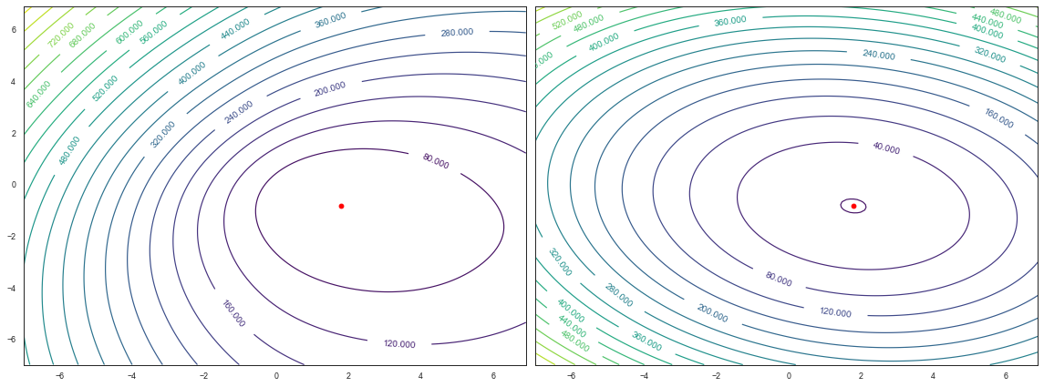
So our Laplace approximation has done a reasonable job. The contours of approximation are at least visually similar to our real posterior. The approximation has also correctly captured that there is more uncertainty in $w_0$ (the x-axis) than $w_1$ which we can see by the broader bowl in the x-axis. Of course, being quadratic, the Laplace approximation cannot capture the asymmetry in the log posterior, but overall it’s not bad!

Issues with the Laplace approximation

Naturally, any approximation method is going to have issues, especially one which assumes quadratic posteriors. Let’s explore the primary weakness of the Laplace method by making a silly but illustrative change to our model:

def log_posterior_2(w, y, X):
    N = len(w)
    w_p = np.zeros(N)
    w_prior_covariance = np.eye(N)
    y_hat = 1/(1 + np.exp(-X.dot(np.cos(0.4*w)**2)))
    prior = 0.5 * (w - w_p).dot(np.linalg.inv(w_prior_covariance)).dot(w - w_p)
    likelihood = np.sum(y * np.log(y_hat) + (1-y)*np.log(1-y_hat))
    return prior-likelihood

This time we’ll plot the log posterior and approximation in 3d:

from mpl_toolkits import mplot3d
fig = plt.figure(figsize=plt.figaspect(0.5))
ax = fig.add_subplot(1, 2, 1, projection='3d')
ax.view_init(60, 35)
ax.contour3D(w_i0, w_i1, log_posterior_surface, 50, cmap='viridis')
ax.scatter3D(w_map[0], w_map[1],grid_sol[1], color='r')
ax.axis('off')
ax.set_title(r"$-\ln p(z)$")
ax = fig.add_subplot(1, 2, 2, projection='3d')
ax.view_init(60, 35)
ax.contour3D(w_i0, w_i1, neg_log_laplace, 50, cmap='viridis')
ax.scatter3D(w_map[0], w_map[1],-np.log(laplace_surface[1]), color='r')
ax.axis('off')
ax.set_title(r"$-\ln q(z)$")

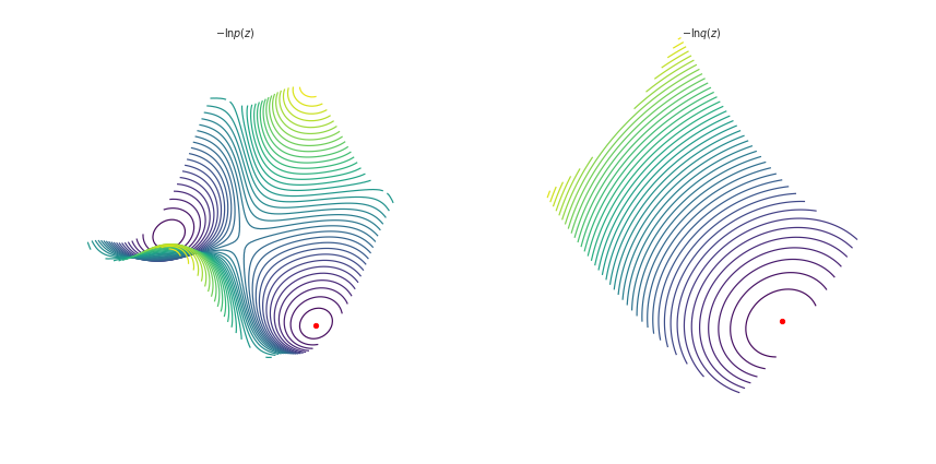
Now our approximation isn’t much good. Our posterior is multi-modal so the MAP isn’t particularly representative, we could equally focus on our Gaussian on the other minima. Our estimate of the variance in the parameters also doesn’t seem particularly good, we’ve not captured the shape of the true posterior at all.