LOWESS (or also referred to as LOESS for locally-weighted scatterplot smoothing) is a non-parametric regression method for smoothing data. But how do we get uncertainties on the curve?

The “non-parametric”-ness of the method refers to the fact that unlike linear or non-linear regression, the model can’t be parameterised – we can’t write the model as the sum of several parametric terms such as with linear regression:

$$ y = \beta_0 + \beta_1 x $$

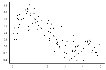
Instead, LOWESS attempts to fit a linear model for each observation based on nearby (or local) observations. This makes the method more versatile than fitting some n-order polynomial to wiggly data but of course, means that we do not have global parameters such as $ \beta_0 $ and $\beta_1$ with which to test hypotheses. To start looking at LOWESS methods, let’s create some nonsense data which has some interesting nonmonotonic response and plot it.

import numpy as np
import matplotlib.pyplot as plt
import seaborn as sns
import matplotlib.pyplot as plt
sns.set_style("white")
plt.rc("axes.spines", top=False, right=False)
sns.set_context("paper")

# make some data
x = 5*np.random.random(100)
y = np.sin(x) * 3*np.exp(-x) + np.random.normal(0, 0.2, 100)
plt.plot(x, y, 'k.')

statsmodels

Python package statsmodels has an efficient LOWESS smoother built-in which provides the obvious choice for doing a lowess smoother in python:

from statsmodels.nonparametric.smoothers_lowess import lowess as  sm_lowess
sm_x, sm_y = sm_lowess(y, x,  frac=1./5., 
                           it=5, return_sorted = True).T
plt.plot(sm_x, sm_y, color='tomato')
plt.plot(x, y, 'k.')

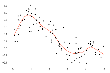
So that looks fairly sensible, sm_lowess has picked out the main structure in the data but not overfitted the curve to any of the noise in the data.

Of course, judging the quality of the fit is difficult because we don’t really have an idea of the uncertainty. Ideally, we’d have a LOWESS method which provides us a confidence interval on the fit of the model so we can see which individual observations are within the fit and those outside of the fitted curve.

Bootstrapping

One obvious way to get a confidence interval around the LOWESS fit is to use bootstrapping to provide an estimate of the spread of the curve. We’ll sample from the observations to change the distribution of points for each fit each time:

import scipy.interpolate

def smooth(x, y, xgrid):
    samples = np.random.choice(len(x), 50, replace=True)
    y_s = y[samples]
    x_s = x[samples]
    y_sm = sm_lowess(y_s,x_s, frac=1./5., it=5,
                     return_sorted = False)
    # regularly sample it onto the grid
    y_grid = scipy.interpolate.interp1d(x_s, y_sm, 
                                        fill_value='extrapolate')(xgrid)
    return y_grid

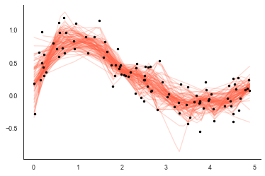
So smooth samples 50% of the observations and fits the LOWESS model. Also because statsmodels doest not provide the solution on an interpolated, and we’re randomly sampling each, the solution is interpolated to the same 1d grid each time specified with xgrid. Let’s run smooth 100 times and plot each lowess solution:

xgrid = np.linspace(x.min(),x.max())
K = 100
smooths = np.stack([smooth(x, y, xgrid) for k in range(K)]).T
plt.plot(xgrid, smooths, color='tomato', alpha=0.25)
plt.plot(x, y, 'k.')

We can then use the individual fits to provide the mean $\mu$ and standard error $\sigma$ of the LOWESS model:

mean = np.nanmean(smooths, axis=1)
stderr = scipy.stats.sem(smooths, axis=1)
stderr = np.nanstd(smooths, axis=1, ddof=0)
# plot it
plt.fill_between(xgrid, mean-1.96*stderr,
                     mean+1.96*stderr, alpha=0.25)
plt.plot(xgrid, mean, color='tomato')
plt.plot(x, y, 'k.')

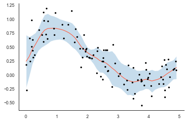
The 95% confidence interval (shaded blue) seems fairly sensible - the uncertainty increases when observations nearby have a large spread (at around x=2) but also at the edges of the plot where the number of observations tends towards zero (at the very edge we only have observations from the left or right to do the smoothing).

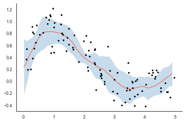
Similarly, because bootstrapping provides draws from the posterior of the LOWESS smooth we can create a true confidence interval from any percentiles:

mean = np.nanmean(smooths, axis=1)
c25 = np.nanpercentile(smooths, 2.5, axis=1) #2.5 percent
c97 = np.nanpercentile(smooths, 97.5, axis=1) # 97.5 percent
# a 95% confidence interval
plt.fill_between(xgrid, mean-1.96*stderr,
                     mean+1.96*stderr, alpha=0.25)
plt.plot(xgrid, mean, color='tomato')
plt.plot(x, y, 'k.')

Writing a custom LOWESS smoother

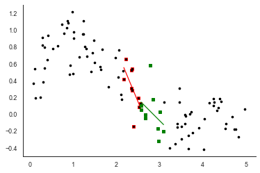
Notice the similarity in the $\mu + 1.96\sigma$ confidence interval and the percentile-based 95% confidence interval. Actually, under certain assumptions about the errors in the data, these should be the same. This is because LOWESS smoothers essentially fit a unique linear regression for every data point by including nearby data points to estimate the slope and intercept. The correlation in nearby data points helps ensure that we get a smooth curve fit. We can understand this a bit more clearly by estimating the curve locally for a couple of observations with linear regression:

import scipy.stats
order = np.argsort(x) # order the points
k = 50
xx = x[order][k-5:k+5]
yy = y[order][k-5:k+5]
plt.plot(x, y, 'k.')
plt.plot(xx, yy, 'rs')
res = scipy.stats.linregress(xx, yy)
plt.plot(xx, res.intercept + res.slope *xx, 'r-')
k = 60
xx = x[order][k-5:k+5]
yy = y[order][k-5:k+5]
plt.plot(x, y, 'k.')
plt.plot(xx, yy, 'gs')
res = scipy.stats.linregress(xx, yy)
plt.plot(xx, res.intercept + res.slope *xx, 'g-')

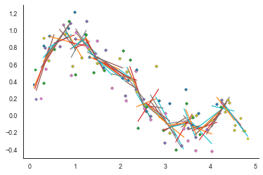
Extending this principle we can get something that looks a bit like the curve from earlier:

order = np.argsort(x)
for k in range(5, len(y)-5 ):
    xx = x[order][k-5:k+5]
    yy = y[order][k-5:k+5]
    plt.plot(xx, yy, '.')
    res = scipy.stats.linregress(xx, yy)
    plt.plot(xx, res.intercept + res.slope *xx, '-')

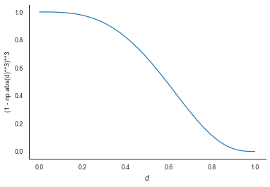
Instead of just selecting the 5 nearest data points and fitting a simple linear regression, LOWESS weights the points based on the proximity of neighbouring points. This is what specifies LOWESS smoothing as just another kernel smoother method in which a function $F$ is used to weight observations based on proximity. For LOWESS, the most commonly used function is the tricube:

tricube = lambda d : (1 - np.abs(d)**3)**3
d = np.linspace(0,1)
plt.plot(d, tricube(d))
plt.xlabel("$d$")
plt.ylabel("(1 - np.abs(d)**3)**3")

Fitting the LOWESS curve

It’s helpful (well necessary) to delve into the LOWESS mathematics at this point. The observations (a collection of x and y points we’ll say) are composed of $x$ and $y$ vectors:

$$ x = [x_1 \cdots x_N] $$

$$ y = [y_1 \cdots y_N] $$

For observation $x_i$, the LOWESS fitting starts with calculating the distance between $x_i$ and each other observation $x_j$ provides:

$$ d_{ij} = [y_{i0} \cdots y_{iN}] $$

With these distances, the tricube weighting function is used to up-weight observations which are more local:

$$ w_i = (1 - |d_{ij}|^3)^3 $$

With $w$ we solve a standard weighted least squares system:

$$ \hat{\beta} = \left(\mathbf{X}^T \mathbf{W} \mathbf{X} \right)^{-1} \mathbf{X}^T \mathbf{W} y $$

where $\mathbf{X}$ is specified as a first order model:

$$ \begin{equation} \mathbf{X} = \begin{bmatrix} 1 & x_1 \\\
\vdots & \vdots \\\
1 & x_N \end{bmatrix} \end{equation} $$

which is a linear model with an intercept (1 values) and the slope. It’s possible to use higher order polynomials of course such as $x^2$ but we’ll stick with the simplest case here. $\mathbf{W}$ is just a diagonal matrix formed from the weights $w_i$:

$$ \mathbf{W} = \begin{bmatrix} w_1 & & \\\
& \ddots & \\\
& & w_N \end{bmatrix} $$

Solving the system provides $\hat{\beta}$ - the intercept $\beta_0$ and slope $\beta_1$. The LOWESS smoothed observation $\hat{y}_{sm}$ is fitted/predicted from the row of the system corresponding to $i$:

$$ \hat{y}_{sm} = \mathbf{X}_i \hat{\beta} $$

So algorithmically we loop over each observation $i$ update the $\mathbf{W}$ with the new weights and resolve the least-squares system above to update $\hat{\beta}$ and then predict each $\hat{y}_{sm}$.

In code this relatively simple to implement for one observation $i$:

dist = np.abs((x[i]-x))
w = tricube(dist)
# form linear system + apply the weights
A = np.stack([w, x*w]).T
b = w * y
ATA = A.T.dot(A)
ATb = A.T.dot(b)
# solve the system
sol = np.linalg.solve(ATA, ATb)
# predict for the observation only
yest = A[i].dot(sol)

Confidence intervals for LOWESS

Because the LOWESS smoother for any individual prediction is essentially weighted linear least squares, the propagation of uncertainty principles are well understood. With any linear model (with normal errors in the observations $y$) the uncertainty in the parameters $var(\hat{\beta})$ are provided from the posterior covariance matrix:

$$\sigma^2\left(\mathbf{X}^T \mathbf{X}\right)^{-1}$$

The diagonal of this matrix provides $var(\hat{\beta})$:

$$ var(\hat{\beta}) = \text{diag} \left[ \sigma^2 \left(\mathbf{X}^T \mathbf{X}\right)^{-1} \right] $$

$\sigma^2$ is important - it is our estimate of the uncertainty in the initial observations. For this approach to work, we are assuming that the observations have an error model of the form:

$$ y = y_\text{true} + \mathcal{N}(0, \sigma^2) $$

The observational error $\sigma^2$ provides an indication of the spread in the observations away from our model of the observations:

$$ \hat{y}_{sm} = f(x) + \epsilon $$

where $f(x)$ is the LOWESS smoothing model and $\epsilon$ is $\mathcal{N}(0, \sigma^2)$ – the error arising in the prediction because of the observations. In some cases, we know what $\sigma^2$ is, but often we don’t. One option to estimate $\sigma^2$ is to assume that our model is perfect and the residuals between the model and observations $(\hat{y}_{sm}-y)$ provides a good estimate. The root mean square error (RMSE) provides this estimate of $\sigma$:

$$ \sigma = \sqrt{\frac{\sum_i^{N}( \hat{y}_{sm} - y_i )^2}{N}} $$

With an estimate of $\sigma$ we can then estimate $var(\hat{\beta})$ correctly and provide a confidence interval based on the assumption that the uncertainty in the parameters is normally distributed. For example a 95 confidence interval on the slope parameter $\hat{\beta_1}$ is:

$$ \text{CI}_{0.95} = \hat{\beta_1} \pm 1.96 \sqrt{var(\hat{\beta_1}) } $$

So we’ve now got a way to get the confidence interval in parameters $\hat{\beta}$ from the variance $var(\hat{\beta})$ but we really want the confidence interval for the fitted curve $\hat{y}_{sm}$.

To get this remember that $\hat{y}_{sm}$ is provided by:

$$ \hat{y}_{sm} = \mathbf{X}_i \hat{\beta} $$

To get the variance or uncertainty in the prediction $var(\hat{y}_{sm})$ we apply standard least squares uncertainty propagation:

$$ var(\hat{y}_{sm}) = var(\mathbf{X}_i \hat{\beta}) = \mathbf{X}_i^T \sigma^2 \left(\mathbf{X}^T \mathbf{X}\right)^{-1} \mathbf{X}_i$$

In code this relatively simple to implement also:

var_y_sm = A[i].dot(sigma**2 * np.linalg.inv(ATA)).dot(A[i])

Wrapping it all up into a lowess function that loops over each observation and fits the curve and uncertainties:

def lowess(x, y, f=1./3.):
    """
    Basic LOWESS smoother with uncertainty. 
    Note:
        - Not robust (so no iteration) and
             only normally distributed errors. 
        - No higher order polynomials d=1 
            so linear smoother.
    """
    # get some paras
    xwidth = f*(x.max()-x.min()) # effective width after reduction factor
    N = len(x) # number of obs
    # Don't assume the data is sorted
    order = np.argsort(x)
    # storage
    y_sm = np.zeros_like(y)
    y_stderr = np.zeros_like(y)
    # define the weigthing function -- clipping too!
    tricube = lambda d : np.clip((1- np.abs(d)**3)**3, 0, 1)
    # run the regression for each observation i
    for i in range(N):
        dist = np.abs((x[order][i]-x[order]))/xwidth
        w = tricube(dist)
        # form linear system with the weights
        A = np.stack([w, x[order]*w]).T
        b = w * y[order]
        ATA = A.T.dot(A)
        ATb = A.T.dot(b)
        # solve the syste
        sol = np.linalg.solve(ATA, ATb)
        # predict for the observation only
        yest = A[i].dot(sol)# equiv of A.dot(yest) just for k
        place = order[i]
        y_sm[place]=yest 
        sigma2 = (np.sum((A.dot(sol) -y [order])**2)/N )
        # Calculate the standard error
        y_stderr[place] = np.sqrt(sigma2 * 
                                A[i].dot(np.linalg.inv(ATA)
                                                    ).dot(A[i]))
    return y_sm, y_stderr

#run it
y_sm, y_std = lowess(x, y, f=1./5.)
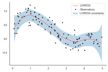
# plot it
plt.plot(x[order], y_sm[order], color='tomato', label='LOWESS')
plt.fill_between(x[order], y_sm[order] - 1.96*y_std[order],
                 y_sm[order] + 1.96*y_std[order], alpha=0.3, label='LOWESS uncertainty')
plt.plot(x, y, 'k.', label='Observations')
plt.legend(loc='best')
#run it
y_sm, y_std = lowess(x, y, f=1./5.)
# plot it
plt.plot(x[order], y_sm[order], color='tomato', label='LOWESS')
plt.fill_between(x[order], y_sm[order] - y_std[order],
                 y_sm[order] + y_std[order], alpha=0.3, label='LOWESS uncertainty')
plt.plot(x, y, 'k.', label='Observations')
plt.legend(loc='best')