Linking python with PostGIS
GIS databases are sort of a necessary evil. Once your data gets too big for RAM you’ve got to start thinking either about relational databases or doing something fancy with dask. PostGIS is a spatial database extender for PostgreSQL object-relational database. In essence, PostGIS puts GIS functions into SQL queries allowing you to run queries and joins based on location. PostgreSQL is big nasty and powerful so this post provides a basic look at utilising PostGIS for the ‘GIS stuff’ and linking python to a PostGIS database for pre-processing and visualisation.
We’ll use the excellent python package osmnx to load some building and land use data from OpenStreetMap.
import osmnx as ox
import matplotlib.pyplot as plt
import geopandas as gp
# get some data
london = (51.501204, 0.001922)
distance=2000
buildings = ox.footprints.footprints_from_point(london, distance=distance)
landuse = ox.footprints.footprints_from_point(london, distance=distance,
 footprint_type='landuse')
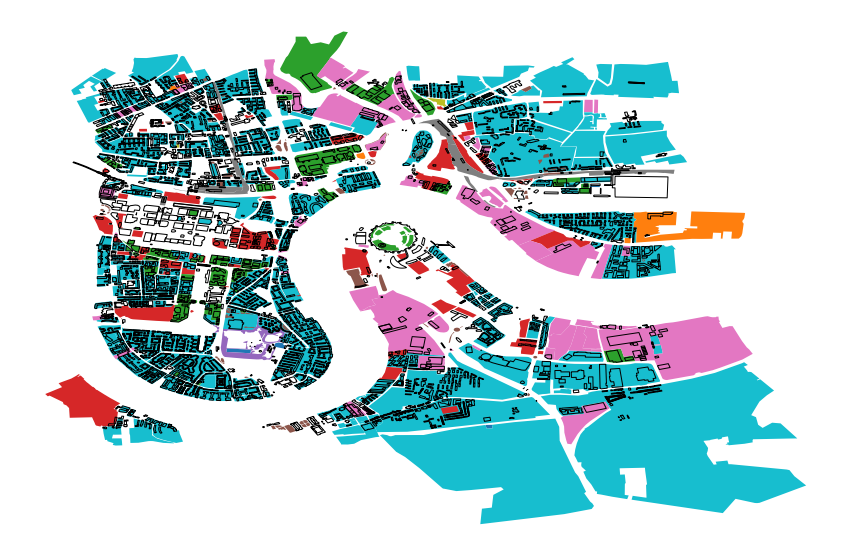
osmnx provides the data back to us in geopandas geodataframes. Let’s make a plot of the data:
fig, ax = plt.subplots(figsize=(15, 15))
landuse.plot(column='landuse', ax=ax)
buildings.plot(ax=ax, color='None',lw=1, alpha=1)
ax.axis('off')
PostGIS
We’ll now dive into Postgres and the PostGIS extension. We can use psql command-line utility for Postgres to execute SQL commands from the terminal to create the database and load the PostGIS extension for Postgres.
➜ psql -U postgres -c "CREATE DATABASE london;"
➜ psql -U postgres -d london -c "CREATE EXTENSION postgis;"
To get the dataframes into the london database I’m going to save them as shapefiles and use the shp2pgsql command-line utility.
(buildings['geometry']).to_file("buildings.shp")
(landuse[['landuse', 'geometry']]).to_file("landuse.shp")
➜ hp2pgsql buildings.shp buildings | psql -U postgres -d london
Looking at the command we can see that shp2pgsql produces a set of SQL instructions which we then pipe to psql to do the actual insertion. If we change the pipe to head we can see the SQL commands that shp2pgsql has generated for us:
➜ shp2pgsql buildings.shp buildings | head


Field fid is an FTDouble with width 11 and precision 0
Shapefile type: Polygon
Postgis type: MULTIPOLYGON[2]
SET CLIENT_ENCODING TO UTF8;
SET STANDARD_CONFORMING_STRINGS TO ON;
BEGIN;
CREATE TABLE "buildings" (gid serial,
"fid" float8);
ALTER TABLE "buildings" ADD PRIMARY KEY (gid);
SELECT AddGeometryColumn('','buildings','geom','0','MULTIPOLYGON',2);
INSERT INTO "buildings" ("fid",geom) VALUES ('0','0106000000010000000103000000010000001300000099709EA0038194BFA40DD1329CC0494002E66BE0586194BFEAFE5657AAC04940010BAA57DB5E94BFAEB25B70ABC04940F3A15577764394BFFC219111ABC049405131CEDF844294BF67ECF07CABC049406B9505B8C5A193BFC742194FA9C049400D068D4FB7A293BFC7B8E2E2A8C04940FF9C386F528793BF15281884A8C049400FE8F120E28B93BFE0EC7B79A6C0494020F8CE1E1E7893BF348FB234A6C04940EBFB15D79D9393BF7CAE00F099C04940DAEB38D961A793BF934CF3339AC04940EA36F28AF1AB93BFB20FB22C98C04940F89F466B56C793BF65A07C8B98C049409A10CE0248C893BFFAD51C2098C049407FAC962A076994BF2E3FCB4E9AC04940DD3B0F93156894BF99092BBA9AC04940EBA463737A8394BF4B9AF5189BC0494099709EA0038194BFA40DD1329CC04940');
INSERT INTO "buildings" ("fid",geom) VALUES ('1','0106000000010000000103000000010000000E0000006778584D7C5A92BFFC4FA335ABC04940E2E7BF07AF5D92BF677627E9ABC04940D08E650B523A92BFB2666490BBC04940C043AC59C23592BF8E76DCF0BBC04940CB64DDE45C2F92BF829A1029BCC049408BBBE6FAE36291BF953F845DB9C049407A956BC0D65B91BFAD252E11B9C0494051DEC7D11C5991BF66A77A8DB8C04940BDDD37633D5A91BF7227220DB8C04940A69C2FF65E7C91BFD3C2C0CEA8C049403C534376398091BF3F4BA13DA8C04940FD3CFCEBCB8891BFC8A4750AA8C0494056945C0F705292BFEA888DC3AAC049406778584D7C5A92BFFC4FA335ABC04940');
INSERT INTO "buildings" ("fid",geom) VALUES ('2','01060000000100000001030000000100000005000000158C4AEA043491BFAB35DE67A6C0494093E4B9BE0F0791BF83723678BAC049408647D1B9916890BF1F85EB51B8C049408341881A3B9790BF59857247A4C04940158C4AEA043491BFAB35DE67A6C04940');
Lets repeat this process for the landuse.shp file:
➜ shp2pgsql landuse.shp landuse | psql -U postgres -d london
And check that the tables have actually been added to the database:
➜ psql -U postgres -d london -c "\dt"

 List of relations
 Schema | Name | Type | Owner
--------+--------------------+-------+----------
 public | buildings | table | postgres
 public | landuse | table | postgres
 public | spatial_ref_sys | table | postgres
(3 rows)
Doing GISy things with PostGIS
Lets now use PostGIS to do some rudimentary GIS analysis. We’re going to look at access to green spaces for the neighbourhood (very roughly!).
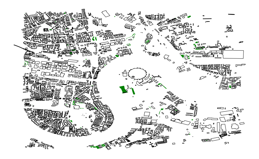
The landuse dataframe defines an associated land use for each polygon. We’re interested only in polygons with an associated grass land use class. Let’s visualise where the grassy areas defined in landuse are:
fig, ax = plt.subplots(figsize=(15, 15))
(landuse[landuse['landuse']=='grass']).plot(column='landuse', ax=ax, color='g')
buildings.plot(ax=ax, color='None',lw=1,alpha=1)
ax.axis('off')
Now, we’ll use PostGIS to do some GISy things which we can then visualise later in python. First, we’ll consider which of the buildings are within 50m of a grassy area. We can construct an SQL query to do this making sure to limit the analysis to only land use polygons where landuse field (landuse.landuse) is grass:
SELECT
 DISTINCT buildings.fid,
 buildings.geom,
 landuse.landuse
FROM
 buildings, landuse
WHERE
 ST_DWithin(buildings.geom::geography, landuse.geom::geography, 50)
 AND landuse.landuse='grass';
So this is a fairly standard looking SQL query - we select fields we need from the two tables buildings and landuse with some constraints as provided by the WHERE. ST_DWithin within is the PostGIS function doing all the work here. It returns true if the geometries are within the specified distance of one another.
The use of the geography keyword buildings.geom::geography is needed because our data is in WGS84 (i.e. latitude/longitude) and we want to do the calculation based on metres. This, of course, means reprojecting the data which is slow so an alternative is to use ST_Distance_Sphere which approximates the calculation in decimal degrees for us. But for good practice and to make the procedure robust to whatever projection the data is in let’s stick with the ::geography transformation here.
Also, the DISTINCT command here is important because it prevents us from storing duplicates of each building (for example when a building is within 50m of more than one grassy geometry).
We can store the query results into a table called within50 by adding an INTO statement:
SELECT
 DISTINCT buildings.fid,
 buildings.geom,
 landuse.landuse
INTO within50
FROM
 buildings, landuse
WHERE
 ST_DWithin(buildings.geom::geography, landuse.geom::geography, 50)
 AND landuse.landuse='grass';
And let’s check the table has been saved:
london=# \dt
 List of relations
 Schema | Name | Type | Owner
--------+--------------------+-------+----------
 public | buildings | table | postgres
 public | landuse | table | postgres
 public | spatial_ref_sys | table | postgres
 public | within50 | table | postgres
(4 rows)
We might wish to generalise this task a bit. How about finding the distance to the nearest grassy area for each building? This an example of a nearest neighbour search. There are several different ways to do a NN search with PostGIS - though unfortunately all of them are a bit involved. I’ve chosen one that hopefully makes some sense:
SELECT buildings.fid,
 ST_Distance(buildings.geom::geography, land.geom::geography) AS dist,
 buildings.geom
INTO buildingsDistances
FROM buildings
JOIN LATERAL (
 SELECT geom, landuse
 FROM landuse
 WHERE ST_DWithin(buildings.geom::geography, geom::geography, 2000)
 AND landuse = 'grass'
 ORDER BY buildings.geom <-> geom
 LIMIT 1
) AS land ON true;
Breaking this down a bit makes the query more digestible. Key to this is query is the LATERAL JOIN method which essentially allows for a join in which the rows of one table are iterated over (as if with a for loop) and the rows matching conditions are then used for the join. The lateral join used here performs the nearest neighbour query and aliases the result as land:
(
 SELECT geom, landuse
 FROM landuse
 WHERE ST_DWithin(buildings.geom::geography, geom::geography, 2000)
 AND landuse = 'grass'
 ORDER BY buildings.geom <-> geom
 LIMIT 1
)
Let’s break this subquery down a bit further. First, we limit the geometries within 2000m of each other. This helps to limit the amount of spatial indexing we’ll do, an efficiency hack essentially. The nearest neighbour search is then effectively done by the following two lines:
 ORDER BY buildings.geom <-> geom
 LIMIT 1
buildings.geom <-> geom is the PostGIS way (termed a “index-based distance operator” of referring to the distance between polygon bounding boxes. This is NOT the same as the true distance between the polygons because it’s based on the PostGIS spatial indexing R-tree (so it’s approximate!). This is what provides the necessary speed to an efficient nearest neighbour search. Then the LIMIT 1 provides only the nearest geometry… nice!
Let’s look at buildingsDistances:
london=# SELECT fid, dist FROM buildingsDistances LIMIT 10;
 fid | dist
-----+--------------
 0 | 539.95580113
 1 | 315.44344397
 2 | 164.43032264
 3 | 4.94973921
 4 | 237.93579893
 5 | 16.53049982
 6 | 79.73473226
 7 | 353.70800526
 8 | 72.46755079
 9 | 231.41497931
(10 rows)
Connecting to PostGIS in python
To create a connection to our PostGIS database from python we can use the versatile sqlalchemy toolkit.
from sqlalchemy import create_engine
db_string = "postgres://postgres:123@localhost:5432/london"
db_connection = create_engine(db_string)
We can execute standard SQL queries which provide back an iterator for the rows of the query:
# check the connection
c = db_connection.execute("SELECT * FROM buildings;")
c.next()
(1, 0.0, ‘0106000000010000000103000077 … (354 characters truncated) … 893BFFAD5CC04940’)
The long string in there is the binary representation of the polygon. Geopandas can connect to our PostGIS database via the from_postgis function with our database connection db_connection:
within50 = gp.GeoDataFrame.from_postgis("SELECT * FROM within50;",
 db_connection,
 geom_col='geom',
 index_col='fid',
 coerce_float=True)
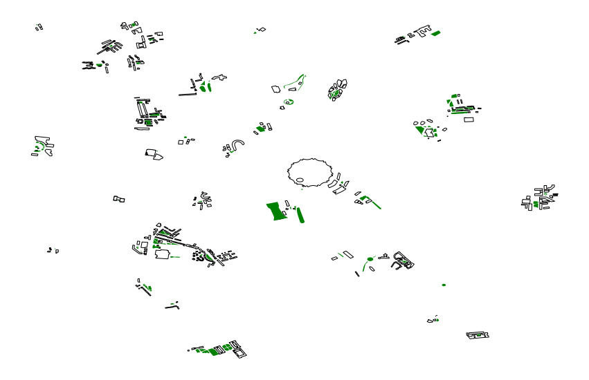
Let’s visualise buildings within 50m of a grassy geometry:
fig, ax = plt.subplots(figsize=(15, 15))
within50.plot(ax=ax, color='None', alpha=1)
(landuse[landuse['landuse']=='grass']).plot(column='landuse', ax=ax, color='g')
ax.axis('off')
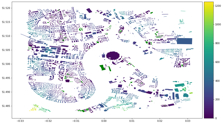
And now let’s visualise the distance for each building:
from mpl_toolkits.axes_grid1 import make_axes_locatable
distances = gp.GeoDataFrame.from_postgis("SELECT * FROM buildingsDistances;", db_connection, geom_col='geom', crs=None, index_col='fid')

fig, ax = plt.subplots(figsize=(15, 15))
divider = make_axes_locatable(ax)
cax = divider.append_axes("right", size="5%", pad=0.1)
im = distances.plot(column='dist',
 cmap='viridis',
 ax=ax, legend=True,
 cax=cax)
(landuse[landuse['landuse']=='grass']).plot(column='landuse',
 ax=ax, color='g')
Further reading
- The official PostGIS workshop is fantastic
- The PostGIS cheat sheet is also pretty good